EME Moonbounce Communication – Getting Started
Successful attempts at bouncing radio signals off the lunar surface were done in 1953, however, the first successful two-way communication was established in the early 1960s. Ever since then, radio amateurs from around the world have been using the lunar surface to establish Earth-Moon-Earth (EME) Moonbounce communication. The earlier contacts were made using slow-speed CW and large antenna arrays were driven by transmitter output of 1 KW or more. Although EME Moonbounce has been attempted even on the 10m and 6m bands, it is more practical and efficient to use the 2m (144 MHz) band all the way up to 10 GHz. With the advancement in available technologies and newer modulation methods, nowadays, effective EME moonbounce is possible with far lesser power and smaller antenna systems. For instance, an 80W 70 cm (432 MHz) setup using about a 12-15 dBi Yagi works well for EME Moonbounce communication using digital modes like the JT65.
Let us, step-by-step, take a look at various challenges posed by EME Moonbounce and how to overcome them. Some of these challenges include the sheer distance between the earth and the moon, the passive reflection from the lunar surface that contributed to losses, the Doppler shift, Libration fading, Echo delays and Time spread, Spatial polarization offset due to curvature of the earth, Cosmic and Galactic noise temperature and background noise, Ionospheric and atmospheric effects like Faraday rotation and Scintillation, etc.
The distance to the Moon and its challenges
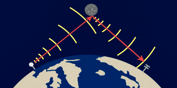
Simplistic depiction of a typical EME moonbounce communication link
Furthermore, the lunar surface is used as a passive reflector, and hence on account of its relatively poor reflection coefficient that is only about 0.065 (6.5%), it drastically attenuates the signal component that bounces off its surface. The low reflection coefficient is largely due to the absorption and scattering characteristics of the lunar surface. Let us see how this translates into the EME moonbounce circuit path loss.
Fundamentally, the propagation path is simple line-of-sight (LOS) and hence the signal strength follows the inverse square law (1/D2). However, since the round trip distance is twice, the signal strength power density at the receiver will be proportionate to 1/D4.
Accounting for the large distance, the lunar surface reflection coefficient, the size of the moon in terms of its disc radius, and the wavelength (λ) of the signal in conjunction with the free-space LOS) attenuation equation that we explained in our article VHF/UHF & Free Space Propagation, we arrive at the following equation that typically specifies the EME moonbounce path loss. For the time being, let us assume that we have Isotropic antennas at both ends of the communication circuit on earth.
 = 10Log({eta r^2 lambda^2}/{64 pi^2 D^4})")
where…
L(dB) is EME free-space path loss with Isotropic antennas.
η is the lunar surface reflection coefficient (0.065).
r is the radius of the moon (1.738 x 10⁶ meters.
D is the distance to the moon (3.844 x 10⁸ meters.
Based on the above equation, the expected magnitudes of path loss of signal power density between two stations on earth may be computed for any frequency band of operation. Though the above-cited earth-moon distance (D) represents the average distance, the slightly different distances during periapsis or apoapsis phases of the lunar orbit may be substituted to find path losses under those conditions. However, we could ignore it for now since the difference is only around ±1.1 dB.
Since the circuit path loss varies as the square of the signal wavelength (λ), prima-facie, it would be correct to conclude that the losses are higher on the higher frequency bands… Here are some of the typical values of EME Moonbounce path losses computed for two-way circuits on various bands.
- 50 MHz (6 m band) — -242.9 dB
- 144 MHz (2 m band) — -252.1 dB
- 432 MHz (70 cm band) — 261.6 dB
- 1296 MHz (23 cm band) — 271.2 dB
- 2304 MHz (13 cm band) — 276.2 dB
Is EME on lower frequency bands easier due to lower loss?
Although, at first sight, it may appear to be true, actually it is just the opposite. Though it may appear to be so from what we calculated above that the EME Moonbounce path loss is around 30 dB less on the 50 MHz (6m) band in comparison to the loss on 1296 MHz (23 cm) band, in real scenarios using real-world antennas, it turns out to be just the opposite. Please remember that our above computations are based on raw path loss parameters with isotropic antennas. If we now add the influence of practical antennas to the above scenario, the overall net path loss trend tends to reverse itself.How do antennas alter the above trend? Let us see…
So far, we noticed that the magnitude of loss is proportionate to λ2. Now, let us assume that the antennas at any end of the circuit were to be of the same physical size irrespective of the frequency band. This would particularly be true in the case of parabolic dish antennas that we often use. It would also be true for other antennas like the Yagi, etc if we were to have similar-sized antennas. The physical size of the antenna practically determines the catchment area of the antenna or what we call as its Effective Aperture.. Keeping the aperture size constant, if we were to alter the frequency, we discover that the gain of the antenna varies as the inverse of the wavelength of the signal (1/λ2). The following equation defines the relationship of the antenna gain and the wavelength for any antenna with a given aperture.
 = 10Log({4 pi A}/lambda^2)")
From the above equation (where A is the aperture), we find that as we reduce the wavelength (increase the frequency), the gain increases as the square of the wavelength (λ). This is the vital factor.
The composite net path loss after accounting for the presence of antennas at both ends now becomes as under…
Lpath(dB) = L(dB) + GT(dB) + GR(dB)
In the above equation, since the antenna gains (GT and GR) of both the antennas contribute with 1/λ2 proportionality, while the free-space loss components contribute only once with λ2, the net effect is to produce a effective path loss which responds to the change in wavelength with 1/λ2 (or proportinate to f2) response.
Since the free-space loss component L(dB) is a negative value and the antenna gains are positive, the outcome of the above equation is to actually produce a smaller negative value that indicates lower overall path loss when the antennas at the earth stations with a given aperture (A) are used at a shorter wavelength or higher frequency… Hence, the fact of the matter is that the higher the frequency band of the EME Moonbounce operation, the lesser is the overall circuit path loss.
Nevertheless, the EME Moonbounce path losses are quite high, in the order of around -250 dB, and thus pose challenges irrespective of the frequency band in use.
Doppler Shift in EME Moonbounce communication
Recognizing and understanding the effects of Doppler shift encountered in EME Moonbounce communication is quite important to the station operator. Like any orbital satellite communication, the continuous change in the relative distance between the orbiting object and the ground station produces the Doppler shift. However, in the case of EME Moonbounce, it is not the orbiting moon that is the major contributor due to a very slow angular velocity of the moon across the sky.
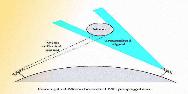
Another depiction of the Earth-Moon-Earth EME moonbounce concept showing how the background galactic noise sources are visible to the antenna due to a much wider beam angle than the angle subtended by the moon.
As the moon ascends above the horizon of the spinning earth, the Doppler shift is maximum and it gradually reduces to zero as the moon appears above the local meridian. Thereafter, the shift changes polarity and behaves like a receding object as the moon traverses the sky till it descends below the horizon. The moon is always available for EME Moonbounce communication irrespective of whether it is optically visible or not as long as it is physically within the line of sight. It does not matter whether it is day or night, or whether it is a full moon or half-moon or whatever.
The magnitude of the Doppler shift is less at lower frequencies and is proportionately higher on the higher frequency bands. The magnitude of the shift is also a function of the latitude of the earth station location and the declination of the moon. Due to the reflective nature of EME Moonbounce communication, the shifts encountered during the upward and the downward legs of signal paths add to produce a cumulative effect. On the 2m (144 MHz) band the Doppler shift could be around 440 Hz whereas on the 23 cm (1296 MHz) it could be as much as 4 kHz. Prima-facie, one might tend to believe that the shift is not much and hence might not pose problems.
However, EME Moonbounce communication, unlike regular satellite radio, do not (or cannot) use the luxury of broader band communication modes like FM or SSB radiotelephony. Due to the colossal path losses, practical EME operation is restricted to narrowband modes like QRS CW or digital modes like JT65, etc. The detection bandwidth needed for communication is very narrow. It may vary from a few hertz to a few tens of hertz. The EME Moonbounce Doppler shift, even though not too much in magnitude becomes significant in proportion to the detection bandwidths of the receivers. The EME station operator would need to keep the narrow receiver detection window continuously tuned to the shifting signal or else the communication link will fail.
Echo Delays, Time Spread and Libration Fading
Recall from the earlier part of this article that the lunar orbit around the earth is slightly eccentric resulting in a slightly elliptical orbit. The difference of distance at the apoapsis and the periapsis is approximately 2592 Km with an average distance being 384104 Km. On account of this and the roundtrip, distance is twice as much, the radio signals traveling at the velocity of light (3 x 10⁸ m/sec) requires about 2.56 sec to be received back on earth. At the Apopsis and the Periapsis of the lunar orbit, the times needed are 2.4 and 2.7 sec respectively. This is known as the EME Moonbounce Echo Delay.
Time Spread
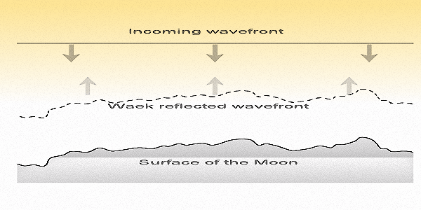
Time spread of the reflected signal caused due to unequal return distance from the lunar surface on account of its surface unevenness.
As a consequence of the time-spreading effect of EME Moonbounce signals, it is not possible to establish error-free communication at high data rates. The inter-symbol spacing between data bits (both CW and Digital) would start merging and overlapping. Hence, for effective and reliable communication it is important to maintain slow data rates to overcome the adverse effects of reflected signal time spread.
The rate of this Libration fading varies with the position of the moon in the sky. Typically, the rate of fading is slower when the moon is near the horizon and becomes maximum as the moon approaches the local meridian. Due to the weak nature of EME Moonbounce signals, the effects of Libration fading needs to be effectively managed to maintain communication reliability. Faster data rates (symbol rate) result in greater communication errors. The slower the data rate, the better is the ability to negotiate the adverse effects of Libration fading. A longer integration time allows the mitigation of faster fading effects.
Coherant Time
At the lower frequency bands like the 2m, the rate of fading is rather slow and it might cycle over a few seconds, whereas, at higher frequencies like the 23 cm or beyond, the fading may occur at the rate of several times per second. The time between fadeouts determines what we call Coherent Time. Due to the longer Coherent time on 2m band, it is more suitable for normal CW while it becomes quite difficult to maintain signal integrity for copying CW on 23 cm band and higher. However, modern digital modulation modes like the JT65 with built-in redundancy, error correction, multi-frequency format, etc are capable of overcoming the effects of intense Libration fading even on the higher microwave bands.Polarization effects due to EME Reflections
In general, at VHF/UHF frequency bands like the 2m or 70 cm, a linear polarized signal that is bounced off the lunar surface retains its polarization. For instance, a horizontally polarized signal from the earth will return back to the originating station with horizontal polarization after the echo delay time. However, circularly polarized signals will reverse their polarization sense. An RHCP signal will return as LHCP and vice-a-versa. Therefore, although it is true that circular polarization w2ill generally experience less fading, the stations using circularly polarized antennas need to be aware of this and need to take the polarization reversal into account.
If we were to conduct EME Moonbounce at higher microwave frequencies, we encounter another phenomenon. The magnitude of this unevenness of the lunar surface appears differently to different wavelengths of the radio frequency. Due to the lack of better resolution at a longer wavelength (lower frequency), the moon appears to be far smoother than how it appears to a shorter wavelength (higher frequency) signal. At 5-10 GHz, the lunar surface appears very rough and uneven resulting in the phenomenon of depolarization due to the moon appearing as electrically a more rough and uneven reflector. The reflected power energy density distributes more evenly across various polarization angles. Hence, the signal received back at earth may be reasonably adequate while using linear polarized antennas as the receiver antenna polarization mismatch may not produce very deep nulls. Of course, there is an overall -3 dB additional attenuation due to this factor.
Spatial Polarization Offset at Earth due to Surface Curvature
The polarization of EME Moonbounce signals received back at a distant location on earth suffers from the effect of spatial polarization offset produced on account of the curvature of the earth. At the microwave frequency range, due to the depolarization of the lunar reflected signal as we discussed above, the effect of spatial polarization offset is less prominent since randomly polarized signals with all polarization angles reach the receiving antenna.
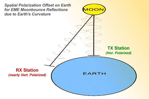
A graphical representation of spatial Polarization Offset experienced between two ends of an EME radio link.
Let us say that at a particular instant in time, an EME station that is located somewhere with the moon aligned with its local meridian. If a horizontally polarized signal from this EME station is bounced back from the lunar surface, it will appear to be horizontally (or vertically) polarized at any other station along the same meridian. However, on account of the curvature of the earth, the polarization of the received signal will be different along different meridians. For instance, if the RX station is longitudinally offset by 45°, then there will be a 45° polarization disorientation experienced by the receiving station antenna. The worst-case scenario will occur when the receiving station location has a 90° meridian offset because the signal received by this station will experience a 90° polarization change. In other words, although the transmitting EME station transmitted a horizontally (or vertically) polarized signal, the RX station at a 90° meridian offset will receive a vertically (or horizontally) polarized signal.
Although I cited an example of meridian offset, the polarization offset may occur with different latitudes also. It would depend on the longitudinal position of the moon vis-a-vis the transmitting station. The compound effect of longitudinal (meridian), as well as latitude offsets, might also occur.
The above would be true if there is nothing else that would influence changes in polarization. However, that is not true. The complexity of the situation is compounded by the fact that Faraday rotation adds to the polarization mismatch even further. Moreover, the magnitude of Faraday rotation is an unpredictable variable.
To overcome the orientation uncertainties of the linearly polarized signals arriving at the receiver during EME Moonbounce communication, the antennas are often set up as Crossed-Yagi with a polarization switch or a polarization diversity arrangement. Such schemes would ensure that the polarization mismatch loss could never be more than -3 dB which is equivalent to the maximum possible 45° mismatch. The additional 3 dB loss margin is accounted for while calculating the link budget of the EME Moonbounce circuit.
A rather complex situation might arise at times due to the combined effect of Faraday rotation and the Spatial Polarization Offset, whereby, communication might be possible only in one direction while the return link may fail. If the spatial offset in one direction is +45°, this offset will be -45° for the return link. Now, if the Faraday rotation were to be +45deg; (applicable both ways), then the link in one direction will suffer +45 -45 = 0° polarization shift, while in the other direction it will be -45 -45 = -90° shift thus resulting in no copy. Various peculiar combinations may occur to pose challenges to EME Moonbounce communication. We will leave it at that for the time being and will cover these phenomena in greater detail in separate articles and posts on this website.
Tropopheric & Ionospheric Effects on EME Moonbounce
Both the Troposphere (lower portion of the atmospheric weather system) and the Ionosphere play a role in EME Moonbounce communication. The quantum of these effects varies with the frequency band that is used. In the VHF/UHF spectrum, the Tropospheric effects are fewer but the Ionosphere plays a significant role. On the other hand, at microwave frequencies beyond 1GHz, the roles are reversed where the Troposphere becomes the major influencer while the Ionosphere gradually takes a back seat.
Tropospharic effects
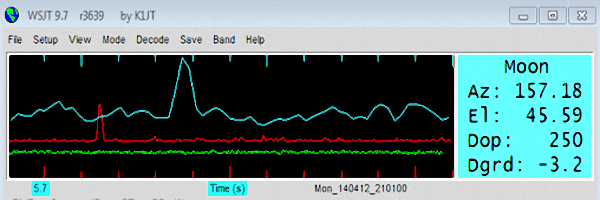
WSJT software panel displaying EME circuit doppler and Link Degradation along with real-time Az/El location parameters from the operator’s QTH.
Higher magnitude of noise at low elevation angles may be the limiting factor at VHF/UHF, whereas, at the microwave region, the absorption of signals due to trees, foliage, and buildings may become quite significant.
The scattering and absorption of radio waves in the microwave segment often become significant. This increases with atmospheric pollutants, dust particles, etc thus contributing to signal attenuation. Raindrops might further attenuate microwave signals making the EME link unstable or even unworkable.
Ionospheric effects
Although the signal attenuation due to the trans-ionospheric propagation is not very significant on the 2m VHF or higher frequency bands, the Ionosphere might modify signal propagation in several ways causing challenges especially in the VHF/UHF region.Other than the Faraday rotation that we have already discussed, the Ionospheric bending of radio waves that penetrate it is a factor that becomes more prominent at shallow angles of incidence. Therefore, when the moon is at a low and moderate elevation above the horizon, the ionospheric bending may result in signals appearing at the EME Moonbounce ground station from a direction that might be different from the visual direction of the moon. Moreover, this signal direction may not be stable and might tend to flicker resulting in rapid signal fading or partial loss. This effect would be more pronounced at VHF compared to UHF or microwave.
Another noteworthy effect that affects an EME Moonbounce circuit is known as Ionospheric Scintillation. Ionospheric scintillations (akin to the twinkling of stars) can play significant roles at VHF and UHF, primarily on EME paths penetrating the nighttime geomagnetic equatorial zone or the auroral regions. The scintillation effect tends to get enhanced during disturbed ionospheric conditions that typically occur during the time of Coronal Mass Ejections (CME) from the sun and is more frequent during the more active part of the 11-year Solar Cycle. The multipath time spread is very small, less than a microsecond, while frequency spread and fading rate can be in the fractional hertz to several hertz. These scintillations can increase the fading rates produced by Earth rotation and lunar librations.
The effects produced by trans-ionospheric penetration are discussed in greater detail in my article on Space Radio Propagation. Please check it out.
Noise Sources as Limiting Factors for EME
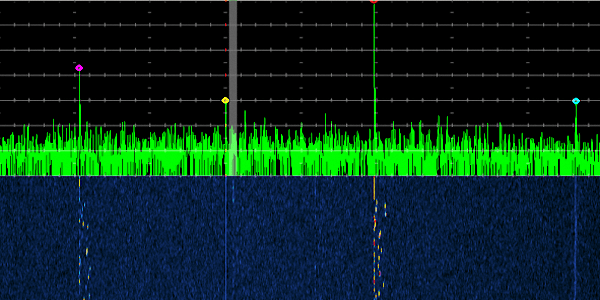
Typical EME signal above the noise floor on the 23 cm band (1296 MHz) displayed on a band scope and waterfall display.
Fundamentally, the received signal level must be greater than the total noise to produce a positive SNR. Failing which, the communication might not be possible. The noise may originate from several sources and their cumulative effect plays up as a spoil-sport. The noise is aggregated over the channel bandwidth (Detection bandwidth) and increases or decreases in proportion to this bandwidth. Therefore the magnitude of the noise is often characterized as noise-power per unit bandwidth (Pn/Hz), where Pn is the noise power. This is termed as the Noise Power Density.
Another way of designating noise magnitude is by specifying it as Noise Temperature. This is a convenient method used while dealing with EME Moonbounce systems. The reason is that many of the EME noise sources are either galactic or originate from large celestial bodies like the sun, the earth, the moon, or the intergalactic space. The noise originating from these sources is traditionally best specified by their noise temperatures. The noise temperature of such sources varies with the frequency band. These celestial objects may appear warmer or colder on different segments of the electromagnetic spectrum.
The Noise Power (Pn) and Noise Temperature (T) have a mathematical relationship and hence may be converted from one to another by the following equation.
")
Where…
Pn = Noise Power in dBW.
k = 1.38 x 10⁻²³ (Botzmann’s Constant in Joules/Kelvin).
T = Temperature in °K (Kelvin).
B = Bandwidth in Hz.
Let us now take a brief look at various noise sources that contribute to EME communication system noise.
Receiver Front-end hardware noise
The radio receiver used for EME Moonbounce communication generates a finite amount of noise on account of the flow of current through various electronic components. The noise contributed by the front-end stages of the receiver plays the most significant role, while the following stages play a progressively lesser role. Hence, the front-end pre-amplifier stage primarily determines the overall noise performance of a well-designed receiver. Nowadays, very low-noise, high-performance semiconductor devices using Gallium Arsenide (GaAs), or Hyper Electron Mobility Transistor (HEMT) devices provide modern receivers with low noise performance that extends well into the microwave region.Tr = 290(10NF/10 – 1)
Where…
Tr = Receiver noise Temperature in °K.
The overall system Noise Temperature (Ts) can be determined by adding Tr to the aggregate of noise from external sources at the antenna input that is designated as Ta.
Ts = Tr + Ta
Thereafter, the overall composite noise referenced to the receiver input may easily be converted back to the RX input Noise Power using the earlier cited equation.
Pn = 10Log(kTsB)
Once the total noise power expected at the receiver input is known, the required transmitter power and the antenna gains needed to establish a viable EME communication link may easily be calculated based on the total path loss and the desired SNR at the receiver.
An EME radio receiver NF of about 1.0-1.2 dB is adequate for 144 MHz band EME due to much higher antenna noise from galactic sources, however, for bands like 70 cm, 23 cm, etc, an RX NF of at least 0.5-0.6 dB is usually better for achieving adequate weak signal performance. Modern small-signal semiconductor devices make this quite possible and are within reach of radio amateurs.
Antenna Noise from Extraneous Sources
The bulk of the noise contribution from extraneous sources that play up in an EME Moonbounce communication scenario come from several natural sources. As we mentioned earlier, the quantum of noise from such sources is frequency-dependent.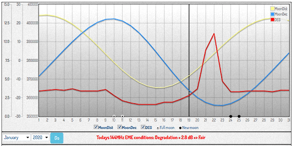
EME link degradation as experienced on 2m (144 MHz) band during the month of January 2020. The Yellow curve shows the variation in distance due to lunar orbit eccentricity, the blue curve shows the variation in declination and the red curve shows the cumulative effect of link degradation in dB over the month.
The lunar phase, its position in the sky, its orbital declination, its position in Apogee/Perigee, etc also influence the overall path loss and the magnitude of composite noise at the RX station EME antenna. These effects are more prominent at lower frequencies like the 2m (144 MHz). The quantum of degradation of the communication link follows a periodic cycle depending on the above factors and the pattern repeats itself every 27.3 days which happens to be the period of a lunar month. The orbit of the moon is inclined with respect to the orbital plane of the solar system. This factor combined with the declination of the earth results in an orbital declination of the moon with respect to the earth. The net effect is that the moon appears to pass across our sky at different latitudes on different days of the lunar month. The maximum swing of its declination is ±28.7° with respect to the earth.
Due to the above-cited reasons, the background celestial bodies and the galactic noise sources that appear behind the moon on different days also vary. On specific days with specific lunar declination, the stronger noise sources from our galaxy (Milky way) might appear in the lunar background. As a result of which the magnitude of antenna noise (especially on 144 MHz and low frequencies) pickup would become much higher than the other days. We call this as EME circuit degradation. During peak degradation days, the net reduction in SNR may suffer by as much as 12-13 dB or more. Due to resource limitations, many amateur EME moonbounce stations that are designed to operate with limited SNR margin would find it impossible to establish EME contacts on these days. Typically, 4-5 days, every lunar month will produce unacceptably high degradations. Just as various satellite pass forecasting software is used to work LEO satellites, there is several moon tracking software available to radio amateurs for forecasting optimal EME operating conditions and days. This makes life easier for EME Moonbounce operators.
Pointer for setting up an Amateur EME Station
In this article, without going into the details of setting up an amateur radio EME station, I will briefly list some of the important factors that need to be kept in mind. I will, however, present details of EME Moonbounce earth station setup and operation in subsequent articles under this section of our website.
Traditionally, over the past decades, CW was primarily used for conducting amateur EME communication. Due to limitations posed by the state-of-art in technology, higher TX power levels, as well as larger antenna arrays, were usually required. Such a setup was usually beyond the reach of most radio amateurs. However, with the advancement in technology, both in terms of available hardware as well as the narrowband digital modulation methods like the JT65, etc, it has now become relatively easy for radio amateurs to pursue EME communication with a limited budget and limited real estate requirements.
Let me present a few pointers on how to get started with EME Moonbounce without breaking the bank, and operating from limited space locations.
- Aim for a station setup for 2m or 70 cm band. 23 cm may also be feasible with some additional equipment.
- A standard amateur radio transceiver that can put out 80-100W on the band of interest.
- Use low loss coaxial cable to connect the antenna like LMR400 or better.
- Install a low noise preamplifier with 0.5-0.8 dB NF at the anteena input point.
- Use at least a 10-12 element Yagi antenna with a boom length of 2-3 λ length.
- Take utmost care to make sure that the antenna has minimum possible side-lobes and other spurious lobes even if it might mean a marginally lower gain.
- Clean lobe pattern will ensure minimum noise pickup from the warm earth and other man-made noise sources at low elevation angle.
- Though there would be a slight increase in noise level at low elevation angles but it would be amply offset by the Gound gain due to the earth.
- To take care of Faraday rotation and Spatial polarization offset, use a Crossed-Yagi (X-pol) antenna configuration with a polarization switch.
- The above scheme will ensure that the polarization mismatch at your receiver is never more than 45° and the loss less than -3 dB at all times.
- Preferably use an Az/El rotator mount with electrial tracking capability. A manually rotatable mount would also suffice.
- Setup the transceiver to work with your computer running a program like WSJT.
- Setup a moon tracking software on your computer, not only to track the moon but also to find the best days of operation with minimal SNR degradation.
EME Moonbounce is after all not as daunting as it may appear to be at first sight. Surely, there are several challenges but a radio amateur who is willing to experiment will find it quite rewarding. I would suggest that a newcomer to EME should start with the minimal setup that I have suggested above. As one gains more experience, one could expand the basic setup and add more punch to the station. At some point, one could also experiment with a more complex LINRAD setup for adaptive polarization compensation and much more. We will speak about LINRAD EME set up in a separate article.


(15 votes, Rating: 5.00) - Please vote the article with your valuable star rating. Thanks! Basu (VU2NSB)

SSN SSNf(10.7) – Real-time Solar Data