Terrestrial VHF Radio Signal Propagation – BLOS
When we refer to beyond-line-of-sight (BLOS) VHF radio communication, we include the non-line-of-sight (NLOS) circuit too. Strictly speaking, NLOS circuits are those which might have been regular LOS path had it not been for some natural or man-made obstacle that came in the way. As per spherical earth geometry, these NLOS paths would be within the radio horizon limits between the two stations. On the other hand, a BLOS communication circuit is essentially beyond the horizon or a trans-horizon circuit. The fundamental difference between the NLOS and BLOS circuit is that in the case of BLOS, it is beside the point whether there may or may not be obstacles in the path in the form of hills, mountains, buildings, etc. However, the path would invariably be obstructed by the terrain bulge of the spherical earth profile.
In this article, I will generally refer to the NLOS circuit as Obstructed Line-of-Sight (Obstructed LOS) for the sake of clarity. As and when a further distinction might need to be drawn, I will qualify the path description by stating if the obstacle under consideration is the terrain bulge or a discrete artifact. Secondly, as we did in the first part of the article series, I will continue to use the term VHF to refer to both VHF and UHF bands from a radio amateur’s perspective.
The Physical Phenomenon of Diffraction – A Knight in Shining Armour
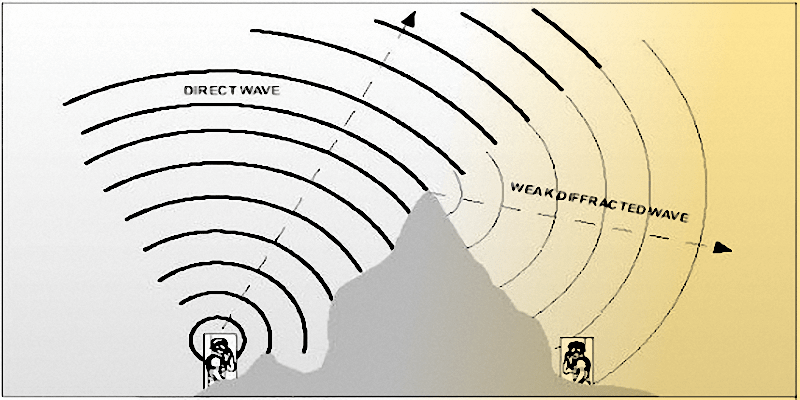
A graphical depiction of the fundamental concept of radio signal diffraction around the edge of an obstacle. Diffraction allows for a part of the radio signal energy to be diverted into the shadow area behind the obstacle.
As we work our way through VHF or higher frequencies, most of their properties begin to resemble those of light waves. Just as a dark shadow is formed when a bright source of light is obstructed, the same happens in the case of a VHF radio signal. If the propagating signals that originated from a VHF/UHF radio transmitter encounter any large object like a building, hill, etc, it casts a radio shadow on the other side of the obstructing object. The radio signals would be blocked by the obstacle thus producing radio darkness (lack of signal) behind it. The receiving stations that lie in the shadow areas beyond such an obstacle will not be able to communicate.
Is there a way by which the VHF radio signal might travel around and behind the obstacle? Thankfully, Yes! … There could be a few workarounds. One way might be that a small amount of radio signal might reach behind the obstacle using multi-path lateral reflections from other objects. This of course is not universally available or may not be a reliable method.
However, the physical phenomenon of diffraction comes to our rescue. Although the diffracted signal strengths that reach into the shadow area, nooks, and corners behind obstacles may not be too strong, they are always consistent under a specific topological scenario. Diffraction allows us communication reliability around corners and in shadow areas.
The trans-horizon BLOS propagation or the obstructed path LOS like the NLOS situation also works primarily due to diffraction.
Essentially, there are two distinct aspects of general terrestrial VHF radio signal propagation. They are the Line-of-Sight (LOS) mode and Beyond-Line-of-sight (BLOS) mode including the NLOS or the obstructed path LOS mode. They both present distinctive traits and attributes. After having examined in detail the clear-path LOS mode of VHF radio signal propagation in the first part of the series, we will now examine both the obstructed path modes including NLOS and BLOS, and also their combined effect in long-range VHF DX communication.
Although to follow this article, it might not be essential to do so, some of the readers might find it interesting to later read through a related article on Atmospheric impact on VHF Radio Propagation.
Obstructed Line-of-Sight (LOS) or NLOS VHF Radio signal Propagation
In the previous article of the 2-part series, we deliberated on typical clear-path LOS VHF radio signal communication. Such a LOS radio communication would be limited to the maximum horizon-to-horizon distance. In such a situation, the 1st Fresnel zone clearance might be violated. However, it is also possible that over shorter distances where the 1st Fresnel zone clearance is preserved, there might be no additional losses. In fact, there might be a perfect 1st Fresnel zone clearance that could lead to a ground reflected gain that could theoretically be as much as 6 dB. However, practically, it would be lesser. Whatever, might be the case, the LOS circuits could either be unobstructed with a clear space in between or there could be one or more man-made or natural topographical obstruction that lies in the path.
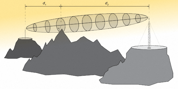
A very basic illustration to depict a situation involving a partial obstruction of the First Fresnel zone region which is shown a a ellipsoidal barrel-shaped virtual space between the two ends of the radio communication circuit.
We are usually interested in the 1st Fresnel zone region though there are n-number of concentric Fresnel zones around the 1st zone. It is only the 1st zone that significantly influences the overall propagation loss. A Fresnel zone is a long ellipsoidal region between the TX and RX antennas. It is an imaginary and intangible region between the two antennas. Any physical object or artifact that lies within this zone could adversely affect propagation in various degrees of magnitude based on the nature and the depth of intrusion.
For our discourse, we will divide the Fresnel zone intrusion region into 2 parts, each representing the nature of intrusion. They are the Reflection region and the Diffraction region. Whenever an obstructing object was to intrudes from any side into the 3-dimensional ellipsoidal Fresnel zone, it begins to affect the signal strength at the receiver end of the communication circuit.
If the amount of intrusion into the Fresnel zone is less than its radius at the place of intrusion, then the obstructing object would not cut off the direct LOS path that runs in a straight line from one antenna to another. Under this condition, the Fresnel zone intrusion is deemed to be in the Reflection region. In this case, the terrestrial VHF radio signal that reaches the RX antenna consists of two components. They are the Direct LOS path signal and the second signal that would be reflected off the top edge (or surface) of the obstructing object. The length of the Direct LOS path and the reflected path is obviously different. Hence, they produce a phase difference between the signals that reach the RX point. Therefore the signals reaching the RX antenna along both these paths would add vectorially to alter the aggregate signal strength at the receiver.
The effective signal strength loss on account of the above phenomena is attributed the to Fresnel zone obstruction of the reflective kind.
Now, if the size of the obstructing object were to be such that it extends deeper into the belly of the Fresnel zone to interrupt the Direct LOS path, then the scenario changes quite dramatically. Although it is still a Fresnel zone obstruction condition, we no more have a direct LOS path, nor do we have a reflection point at the top of the obstruction.
The obstructing object now turns from a reflecting object to a diffracting object. Under these circumstances, the Fresnel zone intrusion is deemed to be in the Diffraction region. In this case, the signal cannot reach the RX station either by direct LOS path or by reflection from an object. The only way the signal might reach the RX is on account of the phenomena of Diffraction from the top of the obstructing object.
Due to quite distinctively different modes of propagation that come into play in the two of the above-cited regions within the 1st Fresnel zone, we will treat these sub-regions separately in the course of our narrative to get a better intuitive understanding. Let us now examine the Fresnel zone Reflection region and the Fresnel zone Diffraction region one by one…
We will assume that the width of the top surface of the obstruction that could be a hill, a building, etc would almost invariably be far smaller in dimension compared to the distance between the TX and the RX radio stations which could be several kilometers or more. Therefore, we will treat the obstruction as a typical knife-edge when we deal with the diffraction situation.
Fresnel zone Reflection region
In typical Fresnel zone reflection region obstruction scenarios, one would always have the line of sight (LOS) direct path between the TX and the RX antennas to be in the clear. The antenna heights are normally more than the height of the obstructing artifact. At least, one antenna at either the TX or the RX end is far taller than the obstruction to ensure a clear direct path between the two.Now, one might ask, what’s the fuss all about? Isn’t a clear path good enough to avoid additional losses? … Well! unfortunately, life isn’t usually so simple.
The ellipsoidal, barrel-shaped Fresnel zone around the path between the two antennas is most often obstructed by the presence of buildings, hills, or other artifacts. If nothing else, then most often it is the protruding curvature of the earth that comes in the way. Any or all of such obstacles may partially cut into the Fresnel zone even though the direct path may be unobstructed. That’s it… This phenomenon of Fresnel zone obstruction is sufficient to result in additional terrestrial VHF signal propagation path losses.
Let us try to explore this intuitively as we build up the narrative…
Fresnel zone obstruction may occur in a reflective mode when the direct line-of-sight LOS path between the two antennas is not interrupted. However, an intrusion by an obstacle in the Fresnel zone will result in some attenuation that will be proportionate to the extent of intrusion.
The calculation of the overall signal in the presence of Fresnel zone obstruction follows a definitive pattern that may be mathematically computed to a fair degree of accuracy. The presence of obstructions at different points along the total path, with varying depth of intrusion into the Fresnel zone envelope, would yield mathematically computable magnitudes of attenuation that the obstructions might cause.
we will come to the computational part later, however, for the moment let us continue to further explore the concept intuitively.
The reflection process that occurs from the top of the obstruction is dictated by several other variables. For instance, all reflecting surfaces are not similar in their smoothness or their reflectivity. Moreover, the obstruction may not always be due to discrete objects like buildings or hills. They may be due to the earth’s bulge which produced an extended obstruction across a large distance along the signal path.
To further complicate matters, the reflection behavior of a radio signal is also dependent on the frequency of the signal, and more importantly on its polarization and angle of incidence on the reflecting surface. The horizontally polarized signal will always undergo 180° phase reversal when reflected from a surface, whereas, in the case of vertically polarized signals, the 180° phase reversal occurs only when the signal strikes the reflecting surface at an angle of incidence of approximately 10° or less. At higher incidence angles, the phase reversal does not occur.
Now, returning our focus to the Fresnel zone, it is interesting to note that its boundary region (Fresnel zone envelope) marks the points at which equal additional attenuation would occur. Within the Fresnel zone envelope, other symmetric and parallel curves can be drawn. Each of these enclosed curves would represent the points of equal magnitude attenuation.
Each of the concentric regions within the boundary of a Fresnel zone outer layer is designated in terms of the Clearance Ratio (or percentage). For instance, a 20% intrusion into the Fresnel zone region is equivalent to 80% clearance, or 40% intrusion as 60% clearance, and so on. The magnitude of attenuation on account of intrusion due to Fresnel zone obstruction would be identical at any value of percentage clearance irrespective of the point of intrusion along the path.
Now, let us broadly see how it pans out under different amounts of intrusions by obstructions into the Fresnel zone region. Let me once again remind you that when we refer to the Fresnel zone in this article, we invariable mean the 1st Fresnel zone.
Here are some vital and seemingly peculiar facts… At 61% clearance (i.e. 39% intrusion), the additionally contributed Fresnel zone loss is 0 dB… Wow! Shouldn’t zero loss be outside the boundary of the Fresnel zone? How can there be no loss when the Fresnel zone boundary has been breached up to almost 40% by the obstructing object?
Well!, what we said above is true. There is no mistake… The fun fact is that when an obstruction is placed at the boundary of the 1st Fresnel zone, it boosts the signal strength at the RX end of the VHF radio communication circuit. The reflected signal from an object located at the Fresnel zone boundary has a path length difference between the direct LOS path and itself which turns out to be 1/2 λ of the signal. This means that the direct and the reflected signal have a 180° phase difference, however, at the reflection point on the obstacle, the signal undergoes another 180° phase shift. The reflection phase shift of 180° always occurs irrespective of the signal polarization in almost all practical situations since the angle of incidence of the signal on the reflecting surface over long-distance circuits is very shallow and most likely be always less than 10°. We discovered this a little while ago in the course of our discussion, didn’t we? Hence, the signals that arrive at the RX antenna along both paths, under this condition, constructively add to enhance the strength. This enhancement is theoretically around +6 dB.
In other words, although we might have initially believed the Fresnel zone boundary to be the point of the start of attenuation, it turns out that it is actually a place where the signal gets boosted. In general radio communication parlance, this is often called the Ground Gain. Usually, with antennas at reasonably good heights, the surface of the earth below might often be placed in a way to produce the additional Ground Gain.
Therefore, if the obstruction is placed at the boundary at 100% clearance point (0% intrusion), we get +6 dB gain. As we begin to intrude with the obstruction penetrating the Fresnel zone, the +6 dB gain begins to diminish, till it becomes 0 dB at 61% clearance. This is the reason why even though the obstacle intrudes as much as nearly 40% into the Fresnel zone, the loss is zero.
If the obstacle were to be taller and intrude deeper into the Fresnel zone region, the attenuation begins to increase, until it becomes theoretically equal to -6.9 dB when the tip of the obstacle is tangentially touching the direct LOS path without obstructing it. The 6.9 dB loss cited above is only applicable when the obstructing object has a narrow top surface. However, in the case of broad topped surfaces, this loss figure tangential to the LOS path would be higher, to be as much as 10-15 dB or even more.
Fresnel zone Diffraction region
So far, we examined what happens when an obstruction intrudes up to halfway into the Fresnel Zone region. What if, the obstructing object is tall enough to cut through the direct LOS path and protrude deeper inside the region?Of course, we would face a different physical situation. We will no more have a direct LOS path. It will be completely cut off. Neither will we have a conventional reflective surface to produce an alternate signal path… So, that’s it? … Does it mean that we would no longer be able to communicate? … Oh! No, we have other physical phenomena that play up under this situation. The phenomena of diffraction takes the front seat now.
When the Fresnel zone intrusion interrupts the LOS path by intruding deep beyond the magnitude of the Fresnel zone radius, then it is deemed to be a Diffractive region intrusion. Under such conditions the attenuation might be quite large.
In the case of terrestrial VHF radio signal propagation into the shadow region behind an obstacle, the signal that grazes across the edge of an obstacle would produce some wavelets that would illuminate the region lying in the shadow of the obstacle. The strength of the signal that is available in the shadow region is dependent on several factors including the wavelength (frequency) of the signal, the size, and shape of the obstacle, the sharpness of the edge around which diffraction would need to take place, etc, etc…
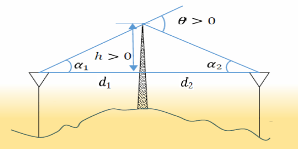
Moreover, the geometry of the diffraction path and the diffraction angle also plays a major role. Refer to the angle marked as θ at the tip of the obstacle in the accompanying illustration. The greater the angle θ the weaker will be the diffracted signal in the shadow region.
This is precisely the principle that applied to the situation of VHF radio signal propagation in dense urban areas that we discussed in the earlier article on Terrestrial VHF Radio Signal Coverage – LOS where we discussed the way VHF radio signal propagates through the urban clutter of a concrete jungle in large cities and metropolises. Diffraction over the top of the buildings, across the city skyline, was the propagation mode where the principles of Fresnel zone obstruction were also applicable.
Since the diffraction loss increases with the angle θ, it is logical to assume that when the obstruction of the intruding object beyond the LOS line of the Fresnel zone is only marginal, then the angle θ would be small and so would be the loss. Therefore, as the intrusion depth increases further, the angle θ also becomes bigger. As a consequence, Fresnel zone obstruction diffraction losses also become greater. The signals at the receiver antenna become weaker.
Therefore, the taller the obstruction between the TX and the RX locations, the greater would be the attenuation. Taller mountains are prone to produce unworkable shadow regions right behind them, while, although a smaller hill might attenuate the signal considerably, yet be strong enough to allow communication. Similarly, the region very close to the foothill on the shadow-side of the mountain might not receive a strong enough signal to make it readable, while moving further away from the foothill, thus lowering the angle θ might suddenly, after a point, allow signal reception to become feasible again.
Let us look a little deeper into this entire process. We will see how the application of the principles of the Fresnel zone defines everything that we discussed above and ties everything neatly into a logical bundle. Not only will it account for obstruction losses due to diffraction but also the reflective type of attenuation that we discussed in the previous sub-section.
The following discourse might be a little more mathematically intense for some of us. However, I suggest that it might be productive if one would attempt to follow through. It will explain the nuts and bolts of how long-distance VHF radio signal propagation works over various obstacles and also over the curvature of the earth’s terrain. In the following section, we will discover ways of calculating Fresnel zone obstruction losses.
In the illustrations associated with the current part of the discussion as well as the previous one related to the Fresnel zone reflection region, we have marked some of the distance and angle variables. Without going into extensive mathematics needed to derive what is known as Fresnel-Kirchhoff Diffraction Parameter (υ) named after the two great scientists who conceived the idea, we will simply state it below and apply it to find magnitudes of Fresnel zone obstruction losses under various conditions of either reflection region or diffraction region obstructions. Simple geometric calculations will suffice for our purpose at this moment.
The Fresnel-Kirchhoff Diffraction Parameter is geometrically specified as under…
υ = h x √((2/λ) x (d1 + d2)/(d1 x d2))
Where…
υ is the calculated Fresnel-Kirchhoff diffraction Parameter.
h is the height of the obstruction in relation to the central LOS path.
λ is the wavelength of the radio signal.
d1 and d2 are the two TX and RX distance from obstacle.
NOTE: Please bear in mind that υ is a dimensionless parameter. The other variables like height, wavelength, and distances must have the same units of measurement. You cannot mix meters and kilometers, or feet and miles, etc. If the wavelength is in meters, then the height of the obstacle as well as bot the TX and RX distances must also be in meters. The height of the obstruction (h) is measured with reference to the central LOS path line. If the top of the obstruction is below the LOS line, as in the case of reflective obstruction, the parameter h is a negative value. On the other hand, if the obstruction cuts through the LOS line, as in the case of a diffractive obstruction, the value of “h” is positive.
Under normal circumstances, the equation for computing the Fresnel-Kirchhoff Diffraction parameter as cited-above is universally applicable. However, in special situations, as in the case of Urban Clutter VHF radio signal propagation over the city skyline by diffraction from the nearby tall buildings, the above equation can be further simplified through acceptable approximations.
In a typical urban clutter propagation under building rooftop diffraction scenario, the two distance is d1 and d2 become grossly asymmetrical thus allowing for the following approximation to be valid. The distance to the nearby building diffraction point d1 is far smaller in the range of few tens of meters, whereas the distance d2 which is the over the skyline distance to the RX far end might be several kilometers (several thousand meters). This means d1 << d2.
If we were to apply an approximation by ignoring the effect of d1 on the sum of d1 and d2 in the numerator of the above equation, it could be simplified to the following…
υ = h x √(2/(λ x d1))
However, please remember that the above simplification is only applicable in the above cited scenario or any similar situation where d1 << d2.
Now that we have derived the Fresnel-Kirchhoff Diffraction Parameter, the rest of it is pretty simple. We will use a fairly accurate approximation for calculating the signal attenuation loss at any diffraction point provided it could be classified as knife-edge diffraction. This should not be a problem under most circumstances since typical man-made obstacles like buildings as well as natural topographical entities often qualify as narrow-topped obstacles. However, there are several exceptions where the diffraction surface may be broad-topped, smooth, or curved. This would lead to a major divergence from a single-point knife-edge diffraction scenario. The bulging curvature of the earth is one such example…
We will cover it in the next section, however, let us first find out how to calculate a typical single-point knife-edge diffraction loss that we might encounter regularly in terrestrial VHF radio signal propagation scenarios. I will present below the equation for computing diffraction loss in decibels (dB). The results from this equation are quite accurate as long as the calculated Fresnel-Kirchhoff Diffraction Parameter (υ) ≥ -0.7. This should be perfectly fine under most practical situations.
L(dB) = 6.9 + 20 x log(√((υ – 0.1)2 + 1) + υ – 0.1)
In many cases when the magnitude of Fresnel-Kirchhoff Diffraction Parameter (υ) is much larger than 0.1, then the above equation may be further simplified without introducing significant error to the following…
L(dB) = 6.9 + 20 x log(√(υ2 + 1) + υ)
In case there are multiple diffraction nodes along the VHF radio signal propagation circuit on account of multiple obstructions situated at different locations, the diffraction loss calculation for each node must be made and then aggregated. In such a situation, the aggregate loss of all diffraction nodes could rapidly increase to unacceptable proportions, especially if the diffraction angle at the nodes is large.
Beyond-Line-of-Sight (BLOS) VHF Radio Signal Propagation over Terrain Bulge
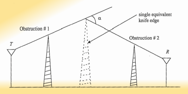
This is an illustration depicting a simplified procedure for finding an equivalent virtual single knife-edge diffraction obstacle that would project similar diffraction loss magnitudes as compared to what might happen in a two cascaded obstacle scenario. This concept helps in simplifying the mathematical equations required to model a terrain bulge attenuation condition.
Rather than falling into the temptation of finding ways of calculating diffraction losses around various arbitrarily shaped geometric objects, let us stay focused on the earth’s terrain bulge. Furthermore, we will avoid complicated mathematical models that might be more accurate but might also be overkill for our purpose. Therefore, I will now present a reasonably good approximation that could be applied to our curved surface earth model. Not only will our method work for the case of terrain bulge but will also be fairly good for estimating diffraction loss across table-top plateaus.
Keep in mind when we speak about terrestrial VHF radio signal propagation over the curved surface of the earth’s terrain bulge we will continue to assume that a standard atmosphere of a normal refractivity gradient is present. In this article, we are not dealing with super-refraction or Tropospheric ducting phenomena that could extend the VHF radio signal coverage over very large distances. I have already covered it separately in the article titled Atmospheric impact on VHF Radio Propagation… Here, we will deal with the phenomena of diffraction that allows for VHF signal propagation around obstacles and curved surfaces even when the Tropospheric refractive gradient remains nominal.
Refer to the associated illustration of an equivalent knife-edge that we could very well approximate when dealing with two or more diffraction points. Although this is an approximation, it is more than accurate for most purposes. If we identify two corner focal points on the surface of the obstacle that would produce a path tangential to the diffraction points, we can geometrically extend the tangent to their point of intersection. This is a virtual point that would now represent a mathematical equivalent of a single obstacle of the derived height, location, and apex angle that would behave very similar to the cumulative diffraction effect that might occur from the two diffraction points at the edge of the obstacle’s surface. Check out the geometry of this approximation in the illustration.
By iteration of the above process, multiple diffraction points on any arbitrary or irregular-shaped obstacle may be converted into a mathematically equivalent single diffraction point. Once we do this, all other calculation processes boil down to a single-point diffraction model. Despite a small degree of error introduced in the process, the final results are accurate enough to be practically acceptable in most scenarios.
In reality, while propagating around a terrain bulge the signal encounters multiple cascaded short-distance diffraction segments along the way. Each of these short diffraction segments is assisted by terrain aberrations. The segment distances, obstacle heights, and diffraction apex angles for each segment are small and hence the diffraction loss contribution of each segment is also small. However, they add up cumulatively in cascade to build up a large total diffraction loss over the curved terrain. Our single point approximation model results in a diffraction loss nearly equal to the aggregate of the above-mentioned segment losses.
I am not going to dwell on elementary school geometry to derive equations for finding the single equivalent virtual knife-edge obstacle that we have discussed but would leave it up to the readers to do the exercise if they wish.
Let us now move forward and try to explore a more realistic real-world VHF radio signal diffraction scenario. Before we look into the curved earth terrain bulge model, let us define a few parameters and also apprise ourselves of a few mathematical equations that would come in handy.
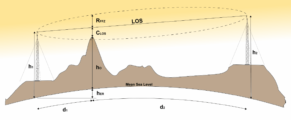
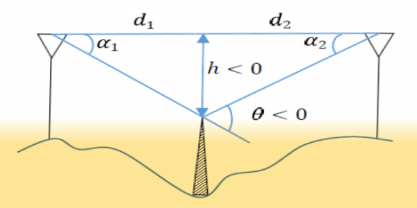
This illustration represents a simplified but realistic Fresnel zone clearance path profile with all required variables marked. This profile will be used to present a set of mathematical equations to be used to calculate various types of VHF propagation losses.
Take a look at the illustration above. It represents a typical point-to-point short-distance LOS propagation path with an obstacle that partially intrudes into the 1st Fresnel zone region of the path. In this example scenario, the antenna heights have been kept different from one another and the obstacle location has been made arbitrary and unsymmetrical. This has been done to account for all the usual typical variables. Furthermore, the curvature of the earth has also been accounted for in this scenario. The additional elevation of the obstacle over-and-above its visible height above ground caused by the curvature of the earth is also taken into account.
All variables that are relevant to our discussion and the set of mathematical equations that follow have been marked on the above illustration. Hence, there should be no ambiguity.
Without further ado, let's roll...
In our narrative, unless explicitly stated otherwise, in every mathematical equations that follow, all distances like d, d1, d2, dOP, etc must be specified in Kilometers, whereas, all wavelengths (λ) or heights like h, h1, h2, hO, hER, RFFZ, CLOS, etc must be specified in meters. This is important because I have for the sake of avoiding confusion normalised several constants like the earth's radius, etc to work with the above stated units of measurements.
Now, here is the first relevant parameter that we would present. It is the Fresnel zone radius (RFFZ). Since the Fresnel zone region is barrel-shaped, the radius at different points along its length will be different. The maximum radius will be midway along the LOS path, while it will gradually reduce as we get closer to the antenna ends.
RFFZ = 31.62 x √(λ x d1 x d2 / (d1 + d2))
Next, let us calculate another parameter, the additional obstacle elevation due to the curvature (hER) caused by the Effective Earth Radius. This parameter is marked as hER in the above illustration.
hER = (d1 x d2) / (12.74 x K)
Where, K is the Effective Earth Radius factor that is determined by the Tropospheric refractivity gradient. For a typical condition under standard atmosphere, K = 1.33. In the case of super-refraction conditions, K > 1.33, while K < 1.33 under sub-refraction conditions would prevail... For typical VHF radio signal propagation scenarios, we work with K = 1.33. However, the set of equations that I am presenting is capable of accounting for any refractivity gradient and hence supports any value of K.
The next step is to calculate the Fresnel zone obstruction clearance distance w.r.t the direct LOS path. This is designated as CLOS in our illustration. To calculate this, the sum total of the obstacle height above terrain (hO) has to be added to hER to find the effective total height of the obstacle. Thereafter, subtract this from the height of the inclined direct LOS path between the antennas at the point of the obstacle location... Getting complicated? ... Don't worry! Here is the combined and simplified equation to find the Fresnel zone clearance CLOS.
CLOS = h1 + ((h2 - h1) x d1 / d) - hER - hO
Earlier in this article, while discussing various types of Obstructed LOS (NLOS) paths, we defined the Fresnel zone obstruction height (h) w.r.t. the direct LOS path between the two antennas that also happens to be the central axis of the Fresnel zone. Any obstruction that intrudes across the LOS path to cutoff the direct path is treated as h > 0, while in the case of the reflective type of Fresnel zone intrusion results in h < 0.
Let us now find out how much would be the Fresnel zone obstruction height in our case. This can be calculated by combining and rearranging the above two equations to yield the following.
h = hO + hER - h1 - ((h2 - h1) x d1 / d)
Please note that the height of the obstacle hO as shown in the illustration applies directly to discrete obstacles like hills, mountains, or buildings. However, in the case of a large curvature like the earth's terrain, hO will be the sum of the Average terrain height AMSL and any additional heights of physical or virtual entities on top of that.
That's all... These were the variables that we needed to derive at this moment... Now, the next step would be to apply the two equations that we had presented earlier to calculate the Fresnel-Kirchhoff Diffraction parameter (υ), and thereafter compute the diffraction loss in dB.
To recap, here are these equations presented once again. Please note that I have introduced a multiplier constant of 0.0316 in the equation below. This is to normalize the distance units to kilometers while retaining the height in meters...
υ = 0.0316 x h x √((2/λ) x (d1 + d2)/(d1 x d2))
and...
LDIFF(dB) = 6.9 + 20 x log(√((υ - 0.1)2 + 1) + υ - 0.1)
If we follow the above sequence of calculations, then we would have no problems in finding the magnitude of the total Fresnel zone diffraction losses in a typical single obstacle terrestrial VHF radio signal propagation circuit assuming a knife-edge diffraction condition.
So far so good...
OK! ... So, are we done? ... No! We are pretty close, but still a few steps away from finding the aggregate Beyond-Line-of-sight (BLOS) propagation loss over the curvature of the terrain bulge. Let's address it right away...
Check out the illustration below. It depicts all major points of interest in a Terrestrial VHF DX Circuit over Terrain Bulge that could be used to proceed further. At the two ends of this terrestrial path, we have our antennas (Ant-1 and Ant-2) which would be at heights h1 and h2 respectively. Due to the terrain bulge along this DX circuit, there is no possibility of direct LOS communication. The direct LOS path (yellow dotted line) between the two stations is buried deep under the earth's surface. The Fresnel zones are also badly breached as can be seen by the white-colored Fresnel zone boundary curves. Hence, the losses, in this hypothetical case would be extremely high and perhaps impractical to overcome. However, please remember that the terrain bulge shown in this illustration is highly exaggerated to highlight the concept. Under normal conditions, due to the huge size of the earth, the effect of curvature is far less.

The illustration shows an exaggerated and not to scale view of a typical scenario that prevails in case of a trans-horizon DX VHF propagation path. The stations are beyon the radio horizon limits and hence a part of the circuit has to negotiate propagation using other means like diffraction over the curved surface of the earth.
Two path segments are unambiguously available for radio signal propagation. They are the radio horizon distances from each of the two antenna locations. These radio horizon points are marked on the illustration. There is clear propagation available from each side up to its associated radio horizon. The balance portion of the overall VHF radio signal propagation circuit that lies in between is obstructed by the pot-belly of the earth. This pot-belly segment would be the diffraction path segment of the circuit.
One might also notice that beyond the radio horizons from each end, the rays have been extended by dotted lines in this illustration to intersect at a point high above in the sky. This point at which these lines meet is our single-point virtual knife-edge diffraction point that we explained earlier.
To calculate the diffraction loss over the extended pot-belly terrain bulge segment of our propagation path, we will use this virtual single diffraction point. To do so, we already have our set of mathematical equations ready to be applied.
However, there is a minor problem that we need to resolve first. As yet, we do not know the height of the virtual equivalent single-point diffraction object. This height is shown on the illustration by a yellow line dropping down from our virtual diffraction point apex and going all the way to the LOS path that is buried inside the earth. We need to find the length of this yellow line that represents the height of the obstruction.
The virtual obstruction height (yellow line) has two parts, the one that is under the surface of the earth, and the other part that is above. We are well equipped to find the length of both these parts and then add them up to find the total virtual obstruction height... How do we do it? ... Not difficult at all, read on...
The part of the virtual height under the surface can be calculated by finding the hER parameter from the equation that we already have with us.
The portion of the virtual obstruction above the surface can be found by a variant of the LOS distance equation that we described in the first part of this 2-part article series that was titled Terrestrial VHF Radio Signal Coverage – LOS.
I will skip the derivations and present the equation as applicable. In our situation, this height will be equivalent to the hO parameter that we assigned for the above-surface obstruction height...
hO = (dOP / (7.14 x K))2 + Average Terrain Height (AMSL)
Where...
dOP is the surface length of the obstructed path due to terrain bulge.
This obstructed path distance (dOP) is equal to the total path length (d) minus the sum total of the two radio horizon distance from each antenna Ant-1 and Ant-2 with heights of h1 and h2 respectively. Therefore...
dOP = d - (3.57 x K √h1n) - (3.57 x K √h2n)
Based on the above, we can now find the magnitudes of d1 and d2 which are the distances from either of the antennas to the point of obstruction.
d1 = (3.57 x K √h1n) + (dOP / 2)
Please note that in the above two equations terms h1n and h2n have been used which are normalised height against the average terrain height Above Mean Sea Level (AMSL). On the other hand, the regular variables h1 and h2 represent heights AMSL.
d2 = d - d1
Applying these to the equation for determining hER will give us the elevation of the portion of the virtual obstacle that is under the surface of the terrain bulge.
At this point, we have all variables ready and available to us to compute the Fresnel-Kirchhoff Diffraction parameter (υ)... This leads to the calculation of the expected diffraction loss along the terrestrial circuit.
Eventually, the total attenuation will be equal to the sum of the free-space loss for the full distance and the diffraction loss. Of course, there would be other smaller losses due to the nature of the earth's surface, vegetation, etc, but their aggregate is far smaller in the case of a VHF DX circuit.
Calculation of Total Terrestrial VHF DX Circuit loss - A Practical Example
Before I conclude this article, let me leave you with a realistic set of calculations as we could apply to practical scenarios. In the example that I cite, the VHF radio signal propagation circuit is a DX path lying in the northern plains of India. We will now analyze the Mussoorie - New Delhi 2m VHF link. Mussoorie is a hill station at the foothills of the Himalayas mountain ranges in the north... BTW, for those interested Himalayas is the home of Mt. Everest too.
From several locations at Mussoorie hills, the northern plains of India present a clear view over a wide-angle that easily allows VHF/UHF DX radio communication into the plains. The practical coverage distance from Mussoorie is along an arc of a radius of 270-300 Km under a standard atmospheric refractivity gradient. Under super-refraction, it could extend by another couple of hundred kilometers. The terrain area coverage for 2m VHF is typically over an arc of 150° and spanning across at least 90,000-100,000 Sq.Km. Here is a map image showing typical coverage.
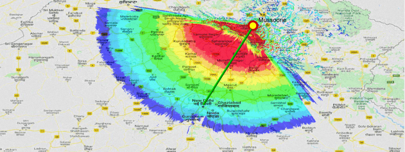
An illustration of 2m band VHF radio signal propagation rendition on a map for wide region covering the northern plains of India. A transmitter (Repeater) is deemed to be located at Mussoorie, India. It provides strong radio signal illumination a region covering many states and cities including my QTH at New Delhi.
In the example below, I will perform link loss calculations for a 2m VHF radio signal propagation circuit between Mussoorie and my (VU2NSB) home QTH in New Delhi, India. Check out the link path profile shown in the illustration below. The illustration marks both ends of the communication circuit on a topographical terrain profile along with the path distance and antenna heights. Here are the path variables that we will use in our example.
- Total Path distance d = 210 Km.
- Terrain height @ Mussoorie = 1783 m AMSL.
- Antenna height @ Mussoorie h1 = 1783 + 3 = 1786 m AMSL.
- Terrain height @ New Delhi = 218 m AMSL.
- Antenna height @ New Delhi h2 = 218 + 28 = 246 m AMSL.
- Average terrain height @ northern plains = 218 m AMSL.
- The radius of Earth = 6371 Km.
- Effective Earth Radius Factor K = 1.33 (4/3).
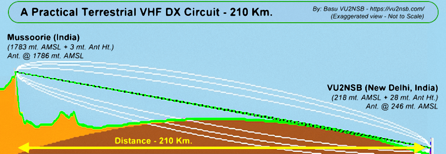
A practical 2m VHF radio signal propagation circuit from the hills of Mussoorie, India to New Delhi, in the northern plains. The path losses including the terrain bulge diffraction loss is calculated for this circuit below. The method of calculation used in this case may be used for finding path losses on any terrestrial VHF or UHF radio communication circuit.
Based on the information provided in the above illustration and the tabulated path data, let us begin our calculations. All calculations are based on the set of equations that we provided above. At this stage, we will apply the relevant equations in a logical sequence to arrive at the final results that we want. Therefore, I will not provide much explanatory narrative in the calculation sequence below. One can always refer back to the previous section of this article in case of confusion... Ready? ... Let's roll...
Radio horizon distance calculations would require the antenna heights to be normalized over the average terrain height.
Radio horizon distance from Ant-1 for a terrain normalized antenna height of 1786 - 218 = 1568 m.
Radio Horizon (Ant-1) = 1.33 x 3.57 x √1568 = 163 Km.
Radio horizon distance from Ant-2 for a terrain normalized antenna height of 246 - 218 = 28 m.
Radio Horizon (Ant-2) = 1.33 x 3.57 x √28 = 22 Km.
Next...
dOP = 210 - 163 - 22 = 25 Km.
Next...
d1 = 163 + 25/2 = 176 Km.
Next...
d2 = 22 + 25/2 = 34 Km.
Next...
hO = (25 / (7.14 x 1.33))2 + 218 = 225 m
Next...
hER = (176 x 34) / (12.74 x 1.33) = 353 m
Next...
h = 225 + 353 - 1786 - ((246 - 1786) x 176 / 210) = 83 m
Next...
υ = 0.0316 x 83 x √(2/2 x (176 + 34)/(176 x 34)) = 0.49
finally...
LDIFF(dB) = 6.9 + 20 x log(√((0.49 - 0.1)2 + 1) + 0.49 - 0.1) = 10.2 dB
We have now got the diffraction loss figure for the 210 Km long VHF radio signal propagation circuit in our example. The diffraction loss computes to approximately 10.2 dB.
To find the total aggregate path loss to expect, let us also add the free-space path loss component for the 210 km long path. We already know from our earlier discussion that Friss Transmission Equation may be applied to do this as under...
Lfree-space = 20 x Log(d) + 20 x Log(f) + 32.4 = 122 dB
If we add the free-space loss, the diffraction loss, and another 5-8 dB miscellaneous loss, then the total VHF radio link attenuation in our example will be...
LossTOT = 10.2 + 122 + 8 = 140.2 ~= 140 dB
This was a real propagation circuit that was used as an example. With a 140 dB path attenuation, excellent communication prospects with strong signals exist. A nominal 5-10W 2m TX will produce a great signal. A 25W base station at both ends with moderate antennas of 1-3 dBi gain would easily produce reliable S9 signals with full quieting on FM.
However, please do not assume that VHF radio signal propagation paths over such long distances would always be possible... No, it won't happen. In this example, the effective height of the antenna at the hill station Mussoorie works out to be 1568m with a clear view of the terrain below.
Using the methods discussed above, attenuation calculations for practical terrestrial VHF radio communication circuits may be made with a fair degree of accuracy.


(18 votes, Rating: 5.00) - Please vote the article with your valuable star rating. Thanks! Basu (VU2NSB)


SSN SSNf(10.7) – Real-time Solar Data