

The Center-fed Half-Wave Resonant Dipole Antenna
A Dipole may present itself to us as the typical stand-alone antenna, or it might also be a part of more complex antennas, very often playing a role as their core sub-component. For instance, an awesome looking multi-element Yagi or even a Cubical Quad antenna are actually formed out of a combination of a set of Dipole elements… Surprised? Nevertheless, it’s true. A dipole is the core building block of most types of antennas that we are usually familiar with. So, when I say that a Dipole antenna is ubiquitous, I really mean it…
Despite its simplicity, the Half-wave Dipole is an antenna that performs rather well. It is a very efficient antenna with a nicely shaped bi-directional radiation pattern that is often amply suited for a variety of terrestrial radio communication applications. Many newcomers to amateur radio, unfortunately, tend to make the mistake of discounting a Dipole as a trivial antenna and setting out on a quest to search for larger and a more expensive antenna that in their view, might do magic. This is perhaps a common blunder.
Although undoubtedly an antenna with better performance specifications compared to a Dipole will outperform it, but that will happen only when things are done the right way. A poorly setup larger antenna will perform as miserably as a poorly setup Dipole. One must first understand and master the factors that ensure good antenna performance in general. What’s good or bad for a Dipole’s performance is also equally applicable to the bigger antenna. Unless one knows how to optimize the performance of one type of antenna, the chances are that one would have no clue how to optimize the other antenna too.
The point I am trying to make is that if you want to upgrade from an existing well-performing antenna to a bigger one, then it’s fair enough. However, if you want a bigger antenna because you couldn’t get your existing antenna to perform up to its optimal capability, then you would be making a mistake. Unless you figure out how o optimize your existing antenna, then in all probability you won’t be able to optimize your new antenna either.
A Brief Synopsis of the Antenna Features & characteristics
In this article, I will try to cover various aspects of the half-wave resonant dipole antenna including, its geometry, characteristics, performance parameters, the influence of practical surrounding environment where the antenna might be deployed, structural integrity, and also some important tips related to its construction as well as transmission line interfacing… Take a quick look at the summary below before we proceed further. The indicated Power Gain is TX mode gain that factors in the overall Radiation Efficiency of the antenna installation. RDF stands for Receive Directivity Factor and it characterizes the antenna receive performance. Radiation efficiency takes into account all structural losses and also ground reflection and absorption losses when applicable.
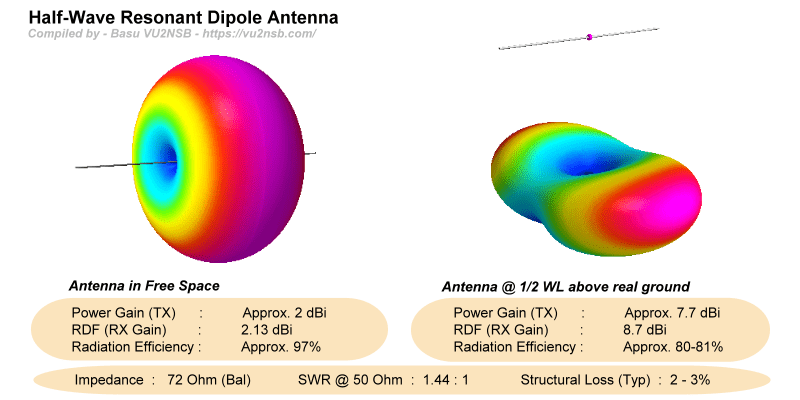
Going by the above summary, it is quite evident that a Half-wave Resonant Dipole is potentially a good antenna that offers high radiation efficiency and also a substantial gain. Despite all these positives, most Dipole installations that fail to deliver satisfactory performance are usually due to reckless installation and deployment.
While installing a rotatable multi-element Yagi, one would give it a lot of thought, especially related to the location of the tower, height above ground, clearance in all directions around the antenna, etc. How often do we do as much due diligence to ensure an equally optimum deployment environment while installing a Dipole? Think about it...
Half-Wave Resonant Dipole Antenna Geometry
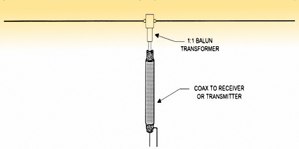
Illustration of a typical Dipole Antenna geometry including a 1:1 Balun to ensure balanced-to-unbalanced transformation of impedance between the antenna and the coaxial cable transmission line.
The principles of radiation from a Dipole are explained in the article titled Principles of Radiation. Please check it out for more information. However, over here, at the moment, let us focus on the other aspects like Dipole geometry and physical size.
At this stage, it might be worth reminding what I stated earlier that a Half-Wave Resonant Dipole is a special case of the Dipole species of antennas. There are other variants too. However, this article is only about the half-wave resonant center-fed variety.
A length of the electrical conductor (wire, pipe, rod, tube, etc.) that is equal to 1/2 λ at the desired operating frequency forms the basis of a half-wave Dipole antenna. At the exact 1/2 λ length of resonance, the conductor will have no reactive current flowing on it and hence the impedance at any point along the conductor will be purely resistive. This resistive impedance will be minimum half-way along the length, at the center. In the case of a half-wave dipole, we use this center-point as the feed-point. The feed-point impedance is, therefore, a purely resistive low value that is close enough to the characteristic impedance of popular coaxial cables so as to produce an acceptable SWR.
What should be the length of a Center-fed Resonant Half-Wave Dipole? Let us find out...
Simplistically, one might say that the length could be derived from the frequency-wavelength formula for EM waves.
λ = C / f
Where...
C = 3 x 10⁸ meter/cec.
f = Frequency in Hz.
Applying the above and conerting frequency to MHz (as f(MHz)) will make C = 300 and now λ = 300 / f(MHz). Half wavelength would mean half of the above value.
λ/2 = 150 / f(MHz)
Is that all? No, unfortunately not... There is more to it. The physical wires have a finite thickness in terms of their diameter. Due to the very prominent Skin Effect at RF, the antenna current flows entirely on the outer surface of the conductor. Despite the solid geometry of the wire, the flow of current is over its cylindrical outer surface. The altered geometry of the current flow alters wire inductance and capacitance. In effect, the velocity of transmission of RF current along the Dipole reduces marginally. The λ/2 value calculated above is no more the actual resonant half-wavelength. Being electrically longer by a small amount, the wire dipole that we have so far produces a small additional inductive reactance.
currently, our dipole has a feed-point impedance Zin = 73 + j42.5 Ω. To compensate for this and bring the conductor length back to resonance, it has been for empirically, for typical wire dipole antennas, instead of the 0.5 λ length, we need to use approximately 0.47-0.48 λ length. Hence in the above formula, we need to replace 150 with 142-143. This would provide a good approximation of the required dipole length in meters. To calculate the dipole length in feet, we need to multiply the result in meter by 3.28.
As a result of the above, the total Dipole length (λ/2) may be calculated as under...
L(mt.) = 143 / f(MHz)
or
L(ft.) = 468 / f(MHz)
The Dipole length determined as above is approximate. The exact length for accurate resonant tuning will vary slightly based on a multitude of factors including the surrounding environment, ground clutter, near-field couplings with objects in proximity, height above ground, the diameter of the conductor, its insulation if any, etc. Therefore, while deploying a Dipole it is always advisable to cut the conductor length about 3-4% longer than the calculated length. During the time of final tuning and optimization, gradually trimming the length from both ends in small and equal steps is recommended.
Typical Dipole Antenna Characteristics & Performance
A Half-Wave Center-fed Resonant Dipole is a light-weight, easy to deploy antenna with remarkable efficiency and structural stability even during storms and adverse weather conditions due to fairly low wind-load surface exposure. The electromagnetic radiation pattern of a dipole is donut-shaped in free-space as may be seen above in the feature synopsis section of this article.
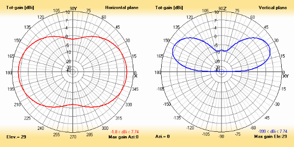
Typical Azimuth and Elevation radiation lobe patterns of a Dipole antenna deployed a 1/2 λ above ground. The Azimuth pattern section is displayed in red while the elevation section is displayed in blue.
The height of the antenna above ground in terms of feet or meters might not always be sufficient to give a real picture. Since various antenna features and performance parameters are a function of the wavelength of the operating signal, the overall performance and the shape of the radiation pattern lobes would more accurately be determined by the height of the antenna in terms of wavelengths (λ) and not absolute values (ft. or mt.).
For instance, an antenna for the 20m HF band might have a certain type of radiation pattern characteristics when installed at a height of 10m above ground which translates to 1/2 λ high above the ground. Now, instead of the 20m dipole, if we deploy a 40m band dipole at the same height of 10m above ground as before, the performance of the 40m dipole antenna would be quite different in comparison to what might have been experienced with the 20m band antenna. This is because, the 40m dipole height is only 1/4 λ (10m) in wavelength terms. If we elevate the 40m dipole to 1/2 λ height i.e. 20m above ground, the performance characteristics will become similar to what we had with the 20m band dipole.
A typical dipole for terrestrial communication, deployed above the earth's surface at a reasonable height, will produce a bi-directional radiation pattern. The beamwidth of the dipole lobes in azimuth is fairly broad. The typical azimuth beamwidth would be about 90° (±45°) @ -3 dB cut-off points for a dipole installed at 1/2 λ height above ground. A dipole antenna installed at different heights above ground will result in quite a significant variation of the overall radiation pattern, however, the azimuth beamwidth will alter marginally unless the dipole is installed at a height of 1/4 λ or less above ground.
When he dipole is at a height of 1/2 λ or more, then a figure of eight shaped azimuth lobe pattern is created. The depth of null at the sides (in line with the wire) typically varies from around 10-20 dB depending on height. higher the dipole, the deeper will be the side nulls. However, when the dipole is lowered below 1/2 λ, it progressively begins to lose the side nulls. The azimuth pattern gradually becomes almost omnidirectional below 1/4 λ height.
There are various other implications of a dipole height above ground that significantly determine the suitability of the installation for communication across radio circuits over various distances. For fixed point-to-point HF radio circuits, in many cases, the installation height of the dipole may well be a significant factor to determine the efficacy of the radio link. However, for us, the radio amateurs, who usually desire to communicate around the world, choosing an optimum height for any antenna, especially on DX HF bands between 20-10m may not be a trivial decision.
Barring the well-known adage that antennas that are higher above ground are better for DX due to low radiation take-off angle, most amateur radio operators are oblivious to the finer effects of antenna height and how it might influence HF radio communication in several other ways. We will cover some of these in the next section on the antenna deployment environment.
Influence on Performance due to Deployment Environment
So far, we have covered some important aspects of a generic dipole antenna installation. Now, it is perhaps time for us to a closer look into various practical matters that influence the antenna performance in real-world deployment environments.
For starters, we must realize that all grounds at all locations are not identical. In other words, the quality of the soil or the ground surrounding the antenna over a fairly large area, influence some of its performance parameters. The two main influencers are the soil conductivity and its dielectric constant. The better the soil conductivity and the dielectric constant, the better it is for the overall antenna performance. The ground reflected wave component loses lesser energy in the form of ground absorption and producing stronger radiation lobes that marginally enhance the gain. The lowest elevation lobe is consequently also enhanced resulting in more radiated energy at lo take-off angles thus improving DX prospects.
From the soil parameter perspective, fertile or moist soil is far better than a rocky, sandy, or a dessert soil. Water bodies like lakes are even better, while seas and oceans are the best due to the saline water being most conductive in nature. This is the reason why the DX performance of antennas is far better for installation in coastal areas or on maritime mobile assets. Moreover, the surface-wave (groundwave) propagation range gets greatly enhanced with enhanced soil conductivity.
For terrestrial communication, the diple antenna derives its additional gain over the gain available in free-space due to the effect of a constructive combination of ground reflected wave components. The direct wave and the reflected wave may either combine constructively or destructively at different elevation angles, thus producing multiple elevation lobes above a certain height over ground. The simple principles of geometric interferometry apply.
Let us now see how these elevation lobes manifest themselves in the overall scheme of the radiation pattern of the dipole. We would also examine how these lobes might affect communication prospects at various distances.
Without further ado, let me present a set of typical dipole radiation patterns for installations at various heights above ground. Although most of it might be self-explanatory, I will, however, summarize the important conclusions.
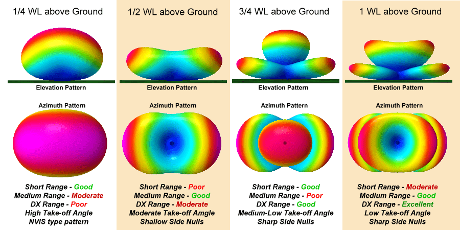
The illustration depicts typical scenarios of Dipole antenna installed at various heights. the effect of the height above ground on the the radiation characteristics of the antenna is shown.
The first case, in our above example at the lefthand vertical column of the illustration, is a Dipole installed at 1/4 λ height above ground. The upper figure represents the elevation section of the lobe pattern, while the lower figure illustrates the azimuth section of the pattern. The expected performance with variation in antenna height is summarized below the figures in each column. The second, third, and fourth columns represent dipoles at heights of 1/2 λ, 3/4 λ, and 1 λ respectively. You can see how the antenna range coverage performance varies drastically with alteration of height above ground. This phenomena is not only unique to a Dipole but is applicable to almost all practical antennas and arrays, barring perhaps vertical antennas that have their own ground plane counterpoise arrangements.
From the above example scenarios, we notice that a dipole that is installed at a lower height (below 1/4 λ) tends to be optimum for short-range communication. The maximum radiated energy is nearly upwards into the sky overhead, thus resulting in more efficient short skips. Such a dipole performs as an NVIS (Near Vertical Incidence Skywave) antenna.
Another important factor to remember about a low height dipole is that the ground soil is in closer proximity resulting in stronger near-field ground coupling. This is a reactive coupling that results in additional loss of RF energy into the earth. The net effect of such n installation is lower antenna efficiency, change in resonant length of the dipole, change in feed-point impedance and SWR, etc. However, a low height (NVIS) antenna is at times desirable to establish short-range HF communication across highly undulating terrain of hills, valleys, gorges, etc, where all else might fail.
Construction Variables and Transmission Line Interface
A typical HF dipole is constructed using a wire conductor, while dipoles for VHF/UHF are usually constructed using aluminum or copper tubings. This apparently makes sense. A typical HF dipole could be several tens of meters long that would perhaps need to be supported at the ends, hence, a length of wire between the two end supports is a logical choice. On the other hand, a VHF/UHF dipole will be short enough to be mechanically self-supporting, hence, a tubing instead of a wire would make it sturdy.
However, there is more to it than the above. As a consequence of the Skin Effect at RF that I have mentioned earlier in this article and also explained in-depth in a separate article, it becomes important to use antenna elements with larger circumference rather than wire conductors at higher VHF/UHF frequencies. A smaller skin-depth at higher frequency means higher RF resistance which in turn would result in greater power dissipation loss in the antenna element thus reducing radiation efficiency.
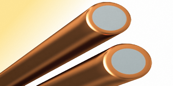
To compensate for the lower skin-depth, the logical alternative is to increase the diameter of the conductor as it increases the circumference thus increasing the overall cross-sectional area and cutting down resistance. The larger diameter conductor need not be solid because RF current flows only on its outer surface. A hollow pipe or tube would serve our purpose equally well, yet be light-weight and cost less.
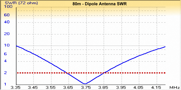
The illustration shows the typical SWR Bandwidth to be expected of a Half-wave Dipole wire antenna on 80m HF band. The fractional bandwidth is typically between 4-6% of the resonant frequency. The bandwidth is more for dipoles with a higher diameter conductor element.
SWR Bandwidth as defined above serves as a yardstick to specify the frequency range over which a resonant dipole would work nicely without the need for Antenna tuning Units (Trans-match). The SWR Bandwidth is directly proportionate to the frequency and may also be expressed in fractional terms. For instance, a 2mm diameter copper conductor (solid or stranded) used to make a 20m band dipole will have an approximate fractional SWR bandwidth of 5.5% which would amount to 0.78 MHz BW. This should be excellent and would suffice to cover the entire allocated amateur radio 20m HF band without the need to use an ATU.
Similarly, on the higher frequency HF bands too, the SWR bandwidth of a dipole made using sufficiently thick conductor should be acceptable. However, on the top bands like 160m or 80m, the SWR Bandwidth is usually no more sufficient. The available bandwidth falls down to about 80-90 KHz on the 160m band, while on the 80m band, it would typically be around 180-190 KHz. Therefore, a full band coverage is not possible with a normal dipole on these top bands. The reduction in bandwidth on the lower frequency bands is further compounded by the fact that the ratio of the element diameter to its length becomes smaller. It is impractical to increase the conductor diameter in proportion to the wavelength.
There are several ways of constructing broader bandwidth dipoles but that's a story for another day. For the moment, we must remember that to attain the maximum possible SWR Bandwidth, try to ensure that the diameter of the element conductor is as high as practically feasible. Thin wire type dipole antennas always compromise not only the antenna bandwidth but also radiation efficiency due to higher accrued resistive losses.
A half-Wave Center-fed Resonant Dipole antenna has a feed-point impedance of 72 Ω and normally would not require an impedance transformer at the feed-point. It can easily interface to the commonly used transmission lines like coaxial cables with Zo = 50-72 Ω. Even with the 50 Ω coaxial cable, the SWR is quite acceptable. However, the dipole is a balanced antenna, while the coaxial cable is unbalanced. Hence, a 1:1 balanced-to-unbalanced RF transformer (BALUN) should be used to achieve the necessary impedance type transformation and prevent unbalancing the antenna and producing common-mode current (CMC) on the transmission line.
The presence of CMC on the transmission line will quite significantly degrade the performance of the dipole antenna. It will cause large RFI during transmit and could also result in unacceptably high noise (QRM) pickup during receive causing a much-elevated noise floor on the HF receiver. Common-mode currents on the feeder must be avoided at all cost. An alternative to the 1:1 Balun is to resort to brute-force choking of the CMC by the use of RF chokes that suppress the CMC. There are several ways of implementing such chokes. Search this website for various articles and posts that deal with this issue.
Important Physical and Structural Aspects of Antenna
While constructing or fabricating an antenna, several important structural aspects ought to be kept in mind. There are several available articles on the internet webspace that provide step-by-step fabrication instructions. They tell you all about antenna dimensions, required components and fixtures like insulators, clamps, bolts, etc. Therefore, I will not go into those aspects.
However, let me touch upon some of the other vital structural aspects that are usually not covered in most of the DIY articles. For instance, what is the type and size of the wire conductor that should be used for a dipole? what are the implications of using either insulated or a bare conductor? How sturdy will be the antenna? How much wind loading due to storms be tolerated by the structure before it fails? etc...
Type of conductor:
A Copper Clad Steel (CCS) wire has a steel core with a thin deposition of copper on the outer layer. CCS wire features a high tensile strength of steel as well as high conductivity of copper. CCS wire is usually used in most professional or critical wire antenna installations.
Copper wires may either be solid single-stranded or be multi-stranded. Both these types may be used for constructing HF wire antennas. However, wire conductors essentially come with two primary types of metal treatment. They are Hard-drawn or Annealed. Hard-drawn copper wire is stronger with higher tensile strength but it is rigid and relatively less flexible than annealed copper wire. Typical copper wire conductors that are available for regular domestic use are annealed wires.
Another special type of wire used for antenna construction is the Copper Clad Steel (CCS) wire. This wire is essentially a steel wire but it has a thin deposition of copper on its surface to form a fused outer layer. The CCS wire offers the best of both worlds. Due to the steel core, it offers the tensile strength of steel, whereas, the outer copper layer offers high electrical conductivity (low resistivity) of copper. For the electrical RF current, the poorer conductivity of the steel core does not matter because, on account of Skin Effect, the RF current restricts itself to the outer surface where there is copper.
The tensile strength of the wire plays an important role in determining its robustness. There are two ways of specifying it. They are the Ultimate Tensile Strength that determines the stress at which the wire breaks after being irreversibly stretched in length. The other parameter is the Yield Strength of the material which determines the stress level beyond which irreversible deformity or damage will begin to occur.
While designing antennas, we are more interested in the Yield Strength of materials to determine acceptable structural stress limits.
I have covered the subject of properties of various materials used for antenna construction in considerable detail in a separate article under the section on Antenna fundamentals. Therefore, for now, let us briefly summarize the properties and application of various types of wires used in antenna construction.
- Annealed Copper - Typical Yield Strength is 33.3 MPa = 3.4 Kgf/mm2. It implies that 2.25 mm diameter wire having 4 mm2 cross-section will be able to sustain a maximum linear stress of 13.6 Kgf (30 lbs), whereas, a 4 mm diameter (12 mm2 cross-section) wire will sustain upto 40.8 Kgf (90 lbs), and so on...
- Hard-Drawn Copper - Typical Yield Strength is 58 MPa = 5.9 Kgf/mm2. It implies that 2.25 mm diameter wire having 4 mm2 cross-section will be able to sustain a maximum linear stress of 23.7 Kgf (52 lbs), whereas, a 4 mm diameter (12 mm2 cross-section) wire will sustain upto 71 Kgf (156 lbs), and so on...
- Copper Clad Steel (CCS) - Typical Yield Strength is 204 MPa = 20.8 Kgf/mm2. It implies that 2.25 mm diameter wire having 4 mm2 cross-section will be able to sustain a maximum linear stress of 83.3 Kgf (183 lbs), whereas, a 4 mm diameter (12 mm2 cross-section) wire will sustain upto 250 Kgf (550 lbs), and so on...
It is important to choose the proper type of wire and also select a proper diameter for the wire antenna application. In the case of top band HF dipole, the choice of wire becomes more important because the dipole length may be large. The dipole needs to be tied between end supports with sufficient tension (tensile force) to prevent undue sag, at the same time, also ensure that the tension does not exceed safe limits.
Effects of Conductor Insulation:
Dipole antennas erected by radio amateurs often use PVC insulated multi-strand copper wire instead of bare wires. This is perfectly acceptable, however, one must bear a few points in mind. First and foremost, it is important to understand that the Velocity Factor (VF) of an insulated wire is always slightly lower than that of bare wire. The difference in VF will depend on the dielectric properties of the insulation as well as its thickness. Typically, this results in shifting the resonant frequency of the dipole to a slightly lower frequency. In other words, if the original length of the dipole was calculated for a bare conductor, then the insulated wire version will need to be shortened a bit to resonate at the same frequency. The typical amount of reduction in length would be approximately 3-5% depending on the material and thickness of the insulation.
Effects of Vageries of Seasons and Weather:
As the season changes, the temperatures also change. This results in linear expansion or contraction of the dipole wire along its length in accordance with the thermal coefficient of linear expansion of the wire material. A dipole that is installed during the summer with a very taut wire may contract during winter thus developing extra tensile stress on the wire. If this stress were to exceed the safe limit, the antenna wire might snap. Moreover, in many countries, during a good part of winter, there might be snowfall. Snow might build upon the dipole wire, presenting a distributed weight across the wire. This would translate to additional tensile stress on the wire which could also lead to a snapped dipole. On the other hand, a dipole wire that is set to a proper tension for winter will result in slack and sag of the dipole wire during summer.
Although the increase in length due to thermal expansion would normally not detune the dipole to a noticeable extent, it is a good idea to take care of the structural issues related to thermal expansion. The simple solution is to tie a dipole wire at one end while keeping it free at the other end. The trick is to run the free-end over a pully and attach a weight to it to keep it under proper tension irrespective of weather conditions. This way, the tensile strength on the wire is always constant and regulated as per one's choice.
Speaking of weather-related issues, some of the other important factors are to ensure protection from the effects of moisture, rain, and UV light. Unless care is taken while building the antenna, both these factors play havoc on any antenna installation over time. Make sure to protect all nonmetallic parts of the antenna from UV light. Either choose UV resistant material or use some kind of protective coating. Rain and moisture-related issues also plague antenna systems. All ends of cables and insulated wires must be protected from seepage or ingress of moisture. The metal joints, screws, bolts, etc must be made of materials that are compatible from the perspective of Galvanic Potential to prevent excessive corrosion. More on Galvanic Potential of metals in a separate article.
Wind Loading and Structural Failure:
A dipole wire antenna on account of its simple structure not much prone to structural failures due to wind loading. Wind loading during big storms, tornadoes, gales, cyclones, etc can be quite catastrophic for large amateur radio antennas. However, designing antennas to withstand storms is an exact science and hence robust antenna structures can be created. Unfortunately, radio amateurs often do not pay enough attention to structural design and therefore leave matters to chance...
In the case of a wire dipole, the typical structural weak-link are h endpoints of antenna wire segments. The stress on the antenna wire due to wind velocity builds up as the square of the velocity. Hence, even with a small increase in wind velocity, the wind force increases rapidly. After a point of increase in wind speed, the force becomes so large as to exceed the yield strength of the wire section. The irreversible elongation of wire occurs at this stage. Thereafter, beyond a point where the Ultimate Yield strength rating is exceeded, the wire would snap at any of its end-points.
Thicker wires even though made out of the same grade of material would be able to survive higher wind velocities. Although the wind loading force increases in proportion to the diameter of the wire, the stress handling limit based on Yield Strength increases as a square of the diameter.


(20 votes, Rating: 5.00) - Please vote the article with your valuable star rating. Thanks! Basu (VU2NSB)


SSN SSNf(10.7) – Real-time Solar Data


