Atmospheric influence on VHF Radio Propagation
Another important factor to keep in mind is that the atmosphere is a very wide region above the earth extending upwards up to 650-900 Km. Within the atmosphere, there are many sub-regions, of which, the Troposphere is the lowest region closest to the earth’s surface. The Tropospheric height varies with latitude, however, on average, it extends from the surface of the earth up to approximately 10-12 Km above. This is the region that contains our weather system including clouds, rain, thunder, lightning, winds, storms, etc… The physical conditions prevailing in the Troposphere are also the factors that impact VHF-UHF Terrestrial Radio communication. Any form of disturbance or anomaly that might occur above the Tropospheric region does not produce any noticeable impact on VHF terrestrial radio. In this article, whenever I might refer to the atmosphere, please understand that we are speaking about the Troposphere. We must also categorically understand that the Ionospheric conditions or Solar activities including SSN, SFI, CME, etc have no impact on terrestrial VHF radio communication systems.
What are the Atmospheric Factors that Influence VHF Radio Propagation?
Before we look into the factors that influence VHF radio propagation on earth, let us first go through those atmospheric (Tropospheric) factors that have very little or no effect on VHF radio.
Firstly, the presence or absence of clouds, rain, lightning, or thunder would rarely be directly responsible for altering VHF radio propagation behavior. At VHF and lower UHF, the raindrops do not produce any significant attenuation. The clouds would not noticeably affect terrestrial communication circuits. At worst, the lightning might produce additional intermittent QRN… All said and done, the VHF radio communication link would generally remain intact.
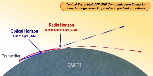
A graphical depiction a typical beyond the optical horizon communication capability of VHF-UHF terrestrial radio communication link under standard homogeneous atmospheric conditions.
At this stage, we must first identify the actual atmospheric parameters that directly affect and mold VHF signal propagation behavior. However, before doing this, we ought to figure out as to what are the common phenomena that play up in the atmospheric region. Once we clarify this, the rest of the jigsaw puzzle will gradually begin to fall in place.
The atmospheric effects in the Tropospheric region tend to deflect the straight Line-of-Sight (LOS) propagation path of VHF-UHF signals. The radio signals start bending gradually along their path. This is what happens. This is the whole story… It is all about how much will the signal paths bend? Or, will it bend at all? If it bends, then in which direction will it bend? Would it bend downwards or will it bend upwards?
These are the million-dollar questions, the answers to which lie in the idiosyncrasies of the atmosphere. The earth itself is spherical. Hence, if the VHF signal transmitted from an antenna were to travel in a straight line without bending, then after a very short distance leading to the optical horizon, it will appear to move away from the curved surface of the earth and escape into outer space. If it were to always happen, we would never be able to operate on VHF-UHF to communicate beyond the optical horizon.
Thankfully, due to several very interesting physical phenomena, the VHF radio signals tend to bend while traveling through the atmosphere. If the bending is downwards along the curvature of the earth, then the communication coverage range gets extended. The magnitude of bending in relation to the earth’s curvature plays a vital role in determining the nature of the overall propagation outcome. However, keep in mind that the atmospheric bending of signals is often a double-edged sword. There might be instances when instead of bending downward, the signals bend upwards. The atmospheric conditions that lead to the upward bending phenomena are mostly undesirable. It shortens the communication range and at times might not even allow communication up to the visible horizon.
All said and done, the bottom line is that the atmospheric influence on VHF-UHF radio communication is primarily all about the bending of propagation paths. That’s it to the whole story…
Now, let us enumerate the atmospheric parameters that are generally responsible for the bending of radio waves. Please remember that this bending phenomenon has an insignificant effect at longer wavelengths like the shortwave HF or MF bands.
Let us recap our understanding of the Ionospheric Skywave Propagation on HF bands. Refer to the article Ionospheric Skywave Propagation to brush up the concepts… Why do the HF radio waves bend back towards the earth after encountering the Ionosphere? That is because the ionospheric layers are comprised of regions of varying (non-constant) Refractive Index. This is called the Refractivity Gradient. Whenever a radio wave encounters a medium with a different refractive index at an oblique angle, it deviates from its original path direction. In the case of a graded refractivity index medium that follows a refractivity index gradient, the bending will continue to occur till the refractivity gradient exists. This is precisely what happens in the case of ionospheric bending of HF signals.
In the case of VHF radio propagation along the earth’s surface, the same phenomena come into play. The only difference is that unlike as in the case of HF ionospheric propagation where the ionospheric refractivity gradient is caused by the variation in plasma density in the ionosphere, in our case of VHF terrestrial signals, it is the Tropospheric region that exhibits the required refractivity gradient that results in VHF signal bending. The density of the air and gasses in the lower Tropospheric region is often different and varies at various heights above ground. This produces a vertical air density gradient starting upwards from the earth’s surface. As we proceed through this article, we will discover that it is this density gradient that causes the bending (either upwards or downwards) of the VHF radio signals.
What are the atmospheric parameters that cause vertical air density gradient that consequently leads to the formation of Refractivity Gradient?
Refractivity Gradient is the most important concept for the purpose of our discussion. I will introduce you to it in a moment… Read on…
Several atmospheric parameters play a role in shaping VHF radio propagation… The air temperature, atmospheric pressure, humidity levels, etc are some of the most prominent factors that are responsible for the creation of Vertical Tropospheric Refractivity Gradient… In the following section, let us examine each of these atmospheric parameters and try to figure out how they collectively influence VHF radio propagation. We will also examine when, how, and where do these phenomena occur.
How is Vertical Tropospheric Refractivity Gradient Produced?
To find out what produces Tropospheric Refractivity Gradient, we will first individually examine three primary atmospheric parameters that are responsible for it. Thereafter, we will find their cumulative effect. We will also study what might happen if one or more of these three major parameters were to suddenly change due to weather system anomalies.
By virtue of the above-cited exercise, we will try to discover the properties of the standard (normal) atmospheric gradients. Thereafter, we will also figure out how various special VHF DX propagation phenomena occur.
Atmospheric Pressure – Variation with Altitude above Ground
If we were to recall what we learned in high-school physics, we might remember that as we move to higher altitudes above the earth’s surface, gradually the air gets rarefied and the atmospheric pressure becomes less. This is also the principle of working of a Barometer.Atmospheric Temperature – Variation with Altitude above Ground
It is also a well-known fact that the temperature of the air becomes lower at higher altitudes. For those who have flown in unpressurized small aircraft, either as a trainee or as hobbyists pilots would know that it progressively gets colder at higher altitudes above the earth’s surface.Atmospheric Humidity – Variation with Altitude above Ground
Humidity in the air is caused by moisture-laden water droplets that might be suspended in the air. This type of moisture content is produced either due to rains or due to clouds that are saturated with water droplets. Or else, elevated humidity in the lower atmosphere near the surface of the earth might also occur as a consequence of evaporation of moisture from the soil or the surface of water bodies like lakes, seas, etc. However, the humidity levels are generally higher near the earth’s surface. As we move to high altitudes, generally the humidity level begins to fall. This is also caused by progressive rarification of air density at higher altitudes.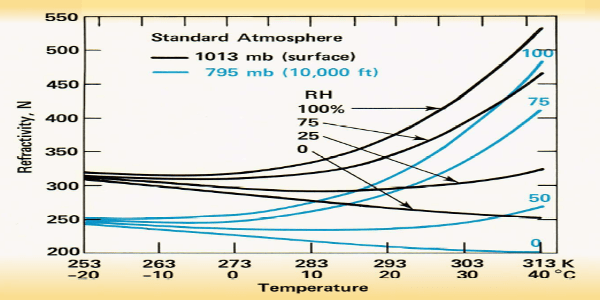
Typical variation of Refractivity (N) of air column under conditions of standard atmosphere based on the variation in pressure, temperature, and humidity. These three influencers ultimately determine the Refractivity Gradient of the Vertical Air column.
Now, that we have decided that the density of air is important, one might ask, why so? A very valid question indeed!!!
The answer to the above question is that when electromagnetic waves, whether it is light, heat, or radio waves travel through any medium, their velocity of travel (propagation) is inversely proportionate to the density of the medium. As the air gets denser, the velocity of radio waves reduces and vice-a-versa. As a corollary one could add that the velocity of radio waves in a vacuum (or outer space) is the highest. However, one must understand that the difference in radio signal velocity in vacuum or air at varying densities is extremely small, but it is enough to produce another related physical phenomenon called refraction.
Refraction occurs when the density of the propagating medium (and consequently the velocity) changes. The refraction property of any medium is quantified and measured by terms called the Refractive Index (n) or Refractivity (N). When two different density mediums like air and water form a transition surface, then the refractivity difference results in the bending of the propagating radio wave away from the straight-line propagation path at the boundary of the two mediums.
In the above paragraph, I cited the example of air-water refractivity boundary transition. However, all refractivity boundaries need not be abrupt as in the above case of heterogeneous mediums. The medium may be a homogeneous medium like a vertical air column, but with a varying air-density gradient along the vertical column. This would produce a gradually varying refractivity index gradient too. Hence, a radio wave that might propagate at an oblique angle through this air column will tend to continually refract the signal and gradually bend the propagation path in a curve.
What we discussed above is precisely what happens in the case of VHF radio signals propagating over the earth’s surface during terrestrial communication… More on this in the next section of the article.
For now, we know that generally, under normal circumstances, the density of the atmospheric air column above the earth’s surface would progressively get rarefied at greater altitudes. Hence, the density would reduce with altitude. Therefore, the Refractivity would also gradually reduce at higher altitudes.
This brings us to another term called the Refractivity Gradient. In our case, we would be interested in the Vertical Refractivity Gradient of the air column of the atmosphere above the earth’s surface. If the refractivity is designated in N-units and the height of the air column in H-units, then if the refractivity gradient would be
ΔN/ΔH
The refractivity gradient is typically measured per unit kilometer height of the atmosphere. Therefore, the Refractivity Gradient is typically specified in ΔN/Km units.
Under most real-world conditions, the Refractivity Index of the air column in the vertical direction above the surface of the earth would gradually reduce with altitude because of lower air density caused by cooler, and less humid air, combined with lower atmospheric pressure at higher altitudes. Therefore, the ΔN part of the Refractivity gradient calculation, as shown above, will be a negative number value. Hence, under normal conditions the Refractivity Gradient specified in ΔN/ΔH or N/Km will be a negative number value.
The average Refractivity Gradient of the vertical air column of the atmosphere above the earth under typical normal weather conditions around the world is statistically found to be -39N/Km. This value of -39 is universally considered as a normal condition and therefore is called the Standard Atmosphere Refractivity Gradient or simply as Standard Atmosphere.
Typical atmospheric Refractivity Gradients and VHF Radio Propagation

Typical manifestation of the conditions of Atmospheric (Tropospheric) refraction. Normal and Super refraction will result in downward bending of the propagating wave thus extending the communication range. Trapping condition is another extreme case of super refraction that allows multi-hop propagation of VHF UHF signals across very long distances. On the other hand, sub-refraction is usually a spoilsport that bends the propagating signal upward and away from the curvature of the earth thus resulting in reduced range.
The magnitude of bending of the propagating radio wave as a consequence of the Refractivity Gradient of the atmosphere is eventually responsible for determining the maximum coverage range for a point-to-point VHF-UHF communication circuit. When the signal propagation path bends significantly enough to follow (or nearly follow) the curvature of the spherical earth, then the communication range gets greatly enhanced. The radio signal will bend along the surface of the earth, well beyond the optical horizon, and travel across a long distance.
Those readers who might be entirely new to the concept of Radio Horizon and Tropospheric bending of Signal Paths might like to first read through my article on Ground Wave Propagation before proceeding further. In that article, I have covered some of the fundamentals along with illustrations…
There are several distinctive types of conditions created as a result of different magnitudes of Refractivity Gradients. Let me list them out below…
- Standard (Normal) Refraction – This is a condition that normally prevails across most parts of the world under average and moderate weather conditions. This happens under the Standard Refractivity Gradient conditions of -39N/Km as defined before. However, refractivity gradients falling near this value in a range between -79N/Km to 0N/Km is often treated as a condition of Near Standard Refraction.
Under these conditions, the VHF-UHF Radio signal bends gradually but slightly towards the surface of the earth. The amount of ray bending is not very significant but it is enough to provide some additional range coverage beyond the optical horizon. The magnitude of range extension of the Radio Horizon is governed by the Refractivity Gradient, from which we derive another factor that we call the Effective Earth Radius Factor designated as K.
Typically, under Standard Atmosphere, the communication coverage range extends by approximately √(4/3) times the optical horizon distance, where the Effective Earth Radius Factor K=4/3. Hence, we usually say that the Radio Horizon is about √(4/3) times or approximately 15.5% further than the optical horizon. - Super Refraction – Under this condition of Super Refraction, the refractivity gradient of the vertical air column typically lies within the range of -157N/Km to -79N/Km. We mentioned in the above section that by definition, the Standard Atmosphere range is till the refractivity gradient of -79N/Km. This is the boundary value at which Super Refraction conditions begin. As this value becomes more and more negative, the propagating radio wave bends more and more downwards towards the earth.
Therefore, due to the greater bending curvature of the propagation path, the signal travels even further beyond the horizon than what happens under Normal (Standard) Atmosphere conditions when the curvature of bending is relatively less. In other words, the phenomena of Super Refraction results in the terrestrial coverage range of VHF radio propagation far beyond what one might expect under normal circumstances, on a regular basis.
The propagation path curvature progressively becomes greater as the refractivity gradient becomes more negative within the Super Refractivity boundary limits. For instance, a typical VHF radio propagation coverage range of say, 50 Km under Standard Refraction might very well extend up to several 100s of kilometers under strong Super Refraction conditions. Such conditions might be for a short period or at times extend up to several hours, or under very rare circumstances, even days at a stretch. - The Magic Gradient [-157N/Km] – Please note the one of the end-points (boundary value) of the Super Refraction range is -157N/Km. This value of the refractivity gradient produces a magical effect. The uniqueness of this condition is that the curvature of the bending of the horizontally propagating radio wave is exactly equal to the curvature of the surface of the earth. In other words, the propagating signal travels parallel to the surface of the earth maintaining an equidistant spacing above the surface all along its path of travel around the spherical earth.
If the refractivity gradient were to be even slightly less negative than -157N/Km, then the signal path’s curvature would be lesser than that of the earth and it would gradually diverge and be lost in space. Similarly, if the gradient were to be more negative than -157N/Km, then it will bend more and strike the earth’s surface after a certain distance.
Since the propagating signal during the Magical Refractivity Gradient condition would run parallel to the surface of the earth, it would not encounter a horizon. A horizon simply would not exist for such a signal. Under this magical condition, the signal propagation would be identical to what one might expect for a flat earth model.
If the magical refractivity gradient were to persist at any time across and remain constant across long horizontal distances around the earth, the VHF radio propagation could become possible across extremely long distances. However, in reality, it does not happen. Due to the dynamic nature of the atmospheric air column and the constantly changing weather system, the magical -157N/Km value does not remain stable and constant for any substantial amount of time. More importantly, this magical value would rarely prevail across a substantial distance along the terrain at any given time. The bottom line is that the magical gradient is usually quite impractical to sustain across a substantially wide stretch of terrain for a long enough duration to conduct a QSO. This exact value of this magical gradient condition is more of an item of academic interest. - Trapping Condition – The magic value of -157N/Km is indeed fascinating but what happens if the refractivity gradient were to become more negative than this magical value? At -157N/Km, the signal was traveling along a curvature that is identical to the curvature of the earth. Hence, the path for VHF radio propagation remained constantly parallel to the earth’s surface.
Now, with the gradient being more negative than -157N/Km, the VHF radio signal will bend even more in the downward direction. Its curvature will be greater than the curvature of the earth. As a consequence, the signal propagation path will be like an inverted parabola. It will continue to bend downwards until it strikes the earth’s surface. Thereafter, it will bounce back (by reflection) to continue its journey ahead. This would lead to the second skip. Multiple cascaded skips could take place to allow the signal to propagate over very long distances.
The effect of the above process may be regarded similar to what occurs during Ionospheric Skywave Propagation of HF radio signals. The difference is that in the case of ionospheric propagation, the ray bending occurs at hundreds of kilometers above the earth, whereas, in this case, the VHF radio propagation signals bend down at far lower altitudes, well below 10 Km in the Tropospheric region. More frequently, this occurs between the ground and up to around 3 Km altitude. The highly negative refractivity gradient of the vertical air column above the earth’s surface is responsible for the VHF-UHF propagation phenomena. This phenomena is called Trapping.
Trapping occurs more often in coastal areas or at other inland places too. However, over the land masses away from the coastal regions, it is more likely to occur after a decent spell of rain, especially after a summer or autumn rain when conditions above ground might become distinctively humid. - Sub Refraction – So far we have examined atmospheric refractivity gradients of various magnitudes and their effect on VHF radio propagation by virtue of the phenomena of signal path bending. However, until now, we have only examined the effects of negative value refractivity gradients. We have yet to find out what happens if this gradient becomes a positive number.
All negative values of refractivity gradients invariably bend the terrestrial propagating radio signal downwards towards the earth. The degree of curvature of ray bending is dependent on the magnitude of the negative gradient. So, what happens if the gradient were to be positive? Does it imply that instead of bending downwards, towards earth, the ray would bend upwards into the sky? … Precisely! That’s exactly what’s going to happen…
The atmospheric conditions that create positive refractivity gradients are generally no good from the perspective of point-to-point terrestrial VHF radio propagation. It ends up in reducing the communication range, at times, by making the coverage range even less than the optical radio horizon distance. This atmospheric condition is called Sub Refraction.
The boundary value between normal (standard) refraction and sub-refraction is the atmospheric refractivity gradient of 0N/Km. At this zero value, the propagating signal travels along a true geometric straight line with absolutely no bending in any direction. However, if the refractivity gradient becomes positive, then upward bending begins to manifest.
The condition of atmospheric sub refraction is a VHF radio communication operator’s nemesis. Unfortunately, such a condition is often a reality. Sub refraction conditions might typically occur on a hot and dry summer day, especially, in a desert or across a rocky land with very little moisture content in the soil.
The concept of Effective Earth Radius Factor – What is it?
The Effective Earth Radius is a notional concept that is designated as K. It is used for performing mathematical computations related to propagation and bending of radio waves…
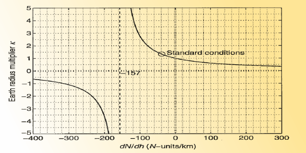
This is a graphical depiction of the relationship between the Refractivity Gradient in N/Km to the Effective Earth Radius Factor (K). K is a simple constant that is easy and more intuitive to apply to mathematical equations to find solutions related to VHF propagation through the atmosphere.
However, due to the refractive bending of radio signals, as we found in our discussion so far, the horizon, from the VHF radio communication operator’s perspective is not the same as the geometric (optical) horizon that we might calculate, given the 6371 Km earth radius. The radio horizon distance would often be longer or shorter (depending on the refractivity gradient) than the geometrically calculated horizon.
So, when we create a mathematical model to analyze or forecast the coverage range of VHF radio communication circuits, we would need to compute a set of mathematical equations that would account for the curving of the radio signal. Only then would we be able to apply it to the earth’s curvature to determine the horizon… Now, we see that it is getting messier. It is no more as simple as finding the geometric horizon by finding a straight line tangential to the circle.
So, is there a way to keep things simple? … Luckily, yes, there is another way that would retain the simplicity, yet would provide accurate results… Fantastic! What is it?
Instead of determining the curved path of the radio wave and thereafter finding its point of contact with the earth’s surface at some point beyond the geometric horizon, how about assuming the signal propagation to be in a straight line but to assume the radius of the earth to be greater or lesser than the physical value of 6371 Km depending on the refractivity gradient value. If we find such an equivalent notional radius that would result in a geometric horizon distance equal to the prevailing radio horizon distance on the real earth, then we would no more need to compute path equations for curving radio waves. We would only need to base our computations on the newly found notional earth radius while maintaining the propagation path as a straight line… This notional earth radius that fits into our mathematical model is called the Effective Earth Radius.
The ratio of the Effective Earth Radius to the Actual Earth Radius is called the Effective Earth Radius Factor and is designated as the constant K. This constant K is now applied wherever required in radio horizon calculations to compensate for the curvature of the bend radio waves and to allow the assumption of the signal path to be a straight line.
So far so good… Now, how do we determine the factor K?
Without going into the complexities of mathematical derivations, I will present below the equation that correlates to the factor K.
K = 157/(157 + ΔN/ΔH)
Where…
K is equal to the Effective Earth Radius Factor.
ΔN/ΔH is equal to the Refractivity Gradient in N/Km.
The Effective Earth Radius Factor (K) plays a vital role in rationalizing various mathematical calculations by allowing us to use general geometric equations. Straight-line tangents and intercepts to a circle work well after having multiplied the actual earth radius with the factor K in any of these equations. This way, we compensate for the curved propagation path caused on account of atmospheric refractive gradients. Radio horizons for Line-of-sight (LOS) or beyond-line-of-Sight (BLOS) paths for VHF radio communication circuits may now be easily characterized. Other important aspects like the Fresnel Zone obstruction losses due to earth’s curvature on a BLOS path and various other propagation parameters can also be calculated after applying the factor K… I have covered this in greater depth in my article titled Path Losses in VHF Terrestrial Radio Circuits. You make check it out at your convenience.
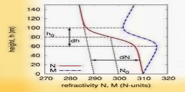
The Modified Refractivity Gradient ((M) is derived from the normal Refractivity gradient that is measured in N-units. This illustration shows a graph with both N-Gradient and M-Gradient plotted side-by-side. It might be a bit confusing to find the ducting conditions from the N-Gradient graph but it is very clearly seen on the M-Gradient curve. A section of the M-Gradient curve that slopes backward is the Ducting region, while the portion of the curve that leans forward represents non-ducting regions.
So far, we have dealt with Refractivity (N) and the Refractivity Gradient (ΔN/ΔH). There is nothing wrong with the above form of specifying these parameters. However, when we present data on various kinds of graphs and charts, we run into a slight inconvenience.
The fact is that at the N-gradient of -157N/Km, the signal propagates parallel to the earth due to the identical curvature of the signal path and the earth. Refer to the earlier part of this article where I explained the Magic Gradient.
Therefore, the -157N/Km value of gradient is unique with reference to an observer on the earth’s surface, since the signal continues to travel parallel to the surface with no path divergence resulting from upward or downward bending. Another way to look at it is to apply the -157N/Km value to the Effective Earth Radius Factor equation above. It computes to infinity. Hence, the Effective Earth Radius would also be infinite. An infinite radius circle (sphere) is essentially a flat surface with no curvature… In other words, the N-Gradient of -157N/Km leads to a Flat surface virtual earth model for this specific condition.
When we draw graphs and charts related to this, then the -157N/Km is an important reference point. Therefore, to make our charts more intuitive and easily readable, it is a good idea to normalize -157 to 0. By doing so, we may easily distinguish between the normal conditions and the trapping conditions that lead to the formation of Tropospheric ducts. Check out the accompanying illustrations.
This is precisely what is done to derive the Modified Refractivity (M) from the well-known Refractivity (N)… Essentially…
M = N + (157 x H)
Where H is the height of the atmospheric layer in Km.
As a corollary to the above, a quick inference that might be drawn from the Modified Refractivity Gradient (M-Grad) is as under…
If ΔM/ΔH < 0, as indicated by the backward sloping trace on a typical M vs H graph, then conditions of inversion resulting in duct formation exists. The backward sloping section might be next to the earth’s surface resulting in a surface duct, or it might occur as a narrow belt of a backward bending slope at a higher altitude. In this case, it would create an elevated duct.
In a graph or a chart, presenting the gradient in terms of M-Grad instead of N-Grad makes it easier to interpret at a glance. For instance, in an altitude vs. gradient graph, if the x-scale is set as M-Grad, then the structure of the trace on the graph easily tells us if there might be a possibility of ducting at any altitude. This would not be so clearly visible if the x-scale of the graph were to be N-Grad. In the case of an M-Grad vs Altitude graph, any portion where the graph trace might bend backward would indicate a suitable region for ducting phenomena to occur.
Anomalous Refractivity Gradient Profiles for VHF Radio Signal Ducting
So far we have discussed the effects on VHF radio propagation caused on account of various conditions of atmospheric refractivity gradient profiles. Whether it was Standard refraction, or Super refraction, or Sub refraction, or whatever, they were all caused by the local weather systems based on the quiescent state of the Tropospheric region.
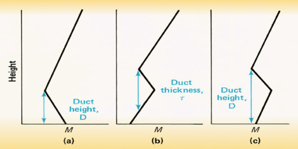
M-Gradient duct profiles in a typical vertical air column of the atmosphere. The profile at (a) indicates a typical Evaporation Duct profile that is formed over the sea, ocean, or large water bodies. The profile at (b) represents the conditions for the formation of the Elevated Duct. The profile at (c) represents a typical surface Duct usually formed by the influx of colder and more humid air near the earth’s surface.
It is not always that a layer of warm air might blow in. It could well be just the opposite where a layer of cold air might come in. The heights above ground at which these weather-front interactive stratifications might occur could vary drastically. These stratifications might occur close to the earth’s surface, or might be several kilometers above. The thickness (in altitude) of these anomalous stratifications might also vary from a few tens of meters to several hundred meters.
For instance, a very warm layer of air at a given altitude might flow in from a nearby location disrupting the smooth vertical refractivity gradient profile that prevailed earlier. With the warm layer of air drifting in, it might cause the refractivity gradient profile to get distorted. We, often refer to such phenomena as Thermal Inversion. A distinct layer with finite thickness, of a larger negative gradient, is created at some altitude above the earth. This may result in the trapping of VHF and UHF radio waves within the bounds of this thermal inversion anomaly. If this were to happen, then an invisible duct of sorts is formed at that altitude above ground.
The VHF radio propagation signals that enter the above described Duct region get trapped within it and travel for very long distances along the duct which behaves like a wave-guide. The signal propagating through such ducts encounters little attenuation. As long as the thermal inversion conditions prevail, the duct mode VHF-UHF propagation phenomena could prevail.

This is a self-explanatory slideshow animation comprising of 5 slides. The first slide depicts a typical standard atmosphere is normal conditions. The second slide depicts a Surface Duct, while the 3rd, 4th, and the 5th, depict Elevated ducting, Evaporation Ducting and Sub-Refraction conditions respectively.
The atmospheric ducting phenomena for radio communication may occur in several ways. Primarily, based on the duct positions, they are categorized as either the Elevated Duct or the Surface Duct.
All such ducts do not behave similarly. Some of them might be well suited for VHF, while others might work fine at UHF but may not sustain VHF. There could be various permutations and combinations of behavior based on atmospheric parameters. As a rule of thumb, the average thickness (in altitude) of the thermal inversion gradient layers that form the ducts, largely determine this behavior. For instance, a duct thickness of about 200m might be sufficient to sustain the ducting of 2m band VHF radio signals, whereas, only about 90m thickness would work perfectly well to trap and propagate 70cm band UHF radio signals, but this duct may not sustain the 2m VHF radio propagation signals. This applies to both forms of ducts, the elevated duct as well as the Surface duct.
Before we proceed further, let me mention that there is a lot of incorrect and misleading information on the World Wide Web, especially related to the formation of Elevated Ducts. Many write-ups and illustrations found on the internet state that a layer of warm air sandwiched between the lower and upper regions of colder air forms the duct thickness. They further go on to state that elevated duct propagation occurs within the confines of the warm air layer boundaries... Such a notion is totally incorrect. Please follow the explanation below and closely refer to the Elevated Duct slide in the above animation.
Elevated Duct
Please refer to the above illustration and check out the slide that depicts a typical Elevated Ducting scenario. This is caused by a layer of warmer air blowing in from an adjacent region that slices into the existing air column. This layer of warm air might form stratification well above the earth's surface. Typically, a majority of these elevated duct forming inversions occur around 3-5 Km above ground, although on rarer occasions, elevated ducts might even form between 1-10 Km altitude.The elevated ducts propagate VHF radio communication signals in the manner shown in the illustration. The propagating radio wave gets trapped or ducted within a region above the earth. As the signal bounces to-and-fro between the duct boundaries, it continues to propagate over very long distances. The signal attenuation (loss) in the elevated duct is extremely small and is governed more-or-less by the inverse square law of free space propagation.
Elevated ducts might occur in various geographic regions under different conditions. However, such ducts form quite frequently in valley regions, where, a layer of air from surrounding higher altitude regions might blow into the valley. This air is usually warmer than the air in the valley. The air while blowing in proximity to the soil in the surrounding higher altitude regions get heated due to the warmer soil. As this layer of air blows into the valley, it creates a warm stratified layer in the air column above the valley, thus marking a suitable condition for elevated propagation ducts.
If you carefully observe the inversion region shown for the elevated duct, you will find that the lower portion of the warm air layer forms the upper boundary of the duct. The lower boundary of the duct is far below, in a region of the vertical air column that is naturally warmer by virtue of its altitude above ground. The duct is the colder region that lies between the naturally warm lower boundary and the upper boundary caused by the warm layer that sliced into the upper part of the air column.
Therefore, the bottom line is that the duct is always the colder air region that is bounded by warmer air layers at the top and bottom as in the case of Elevated Ducts. However, in the case of a Surface Duct, the colder air region is bounded only at the top by a warm layer while the bottom bound is the earth's surface... We will explore it next.
Surface Duct
Surface ducts manifest themselves quite similarly to the conditions of classical trapping caused by the refractivity gradient near the earth's surface caused by a naturally occurring refractive gradient that is more negative than -157N/Km. The classical trapping conditions might require certain very specific local weather conditions to be met. For instance, very high surface level humidity resulting in elevated vapor pressure close to the earth's surface might be needed. It's not always a temperature gradient but at times even a good humidity gradient will produce the required conditions... Remember, in the earlier part of this article, I had explained how three major factors, namely, the temperature, the humidity (vapor pressure), and the atmospheric pressure are all responsible for producing refractivity gradient profiles leading to phenomena like ducting, etc.The key difference between Surface Ducting and the native N-Gradient-based local trapping phenomena is that, unlike local trapping, Surface ducting is not strictly a local phenomenon. It is based on the interaction between the local and another neighboring region weather-front.
Surface Ducting is in principle fairly similar to elevated Ducting. The primary difference is that the altitude of the warm layer ingress into the existing air column is much lower. The inversion layer is typically below 1Km altitude, and most likely to be in the region of 300-500m above ground. As a consequence, there is not enough room below the inversion altitude to form a lower boundary layer to form an elevated air duct. The lower boundary of such a low altitude duct is therefore missing. Hence, the surface of the earth acts as the lower duct boundary. The propagation of radio waves would therefore have to occur within a duct with the upper bound comprising of the thermal inversion while the lower bound is the earth's surface... Hence, it is called a Surface Duct.
Surface Ducts are typically lossier in comparison to elevated ducts. This is due to greater attenuation from each earth's surface reflection. Various physical phenomena like earth surface absorption, scattering, etc come into play to accentuate net attenuation.
On the bright side, the surface ducts are usually easier to exploit for amateur radio communication with far greater regularity than elevated ducts. Though the elevated ducts occur more often at upper UHF and microwave frequencies, they are fairly elusive at VHF radio communication frequencies.
In the case of elevated ducts, I cited an example of a warm layer of air from a neighboring region, cutting in to create a thermal inversion layer. However, it is not always necessary for warm air layers to produce ducts. It might as well be a colder layer of air that might result in the formation of ducts. For instance, a cooler layer of air over the surface of the sea or a large lake might blow into the coastal area during the day when the air temperature over land is usually higher. This colder, denser, and more humid layer of air from the sea would replace the warmer and lighter air that existed near the surface across the coastal land. As a consequence, a typical condition of low altitude thermal inversion would occur, giving rise to a robust surface duct... There could be many other permutations and combinations of vertical air column density gradient stratification. All such conditions would lead to anomalous refractivity gradients that produce anomalous propagation at VHF, UHF, and beyond.
Evaporation Duct
This is a kind of a Surface Duct. However, I felt it necessary to cover it separately due to several of its uniqueness, especially, the phenomena that lead to its creation. Unlike regular surface ducts, the Evaporation Ducts are not produced by the interaction of adjacent region weather-fronts. It is a local phenomena.Although technically evaporation ducts might form to an extent even over land after rains in a hot tropical region, it is primarily a phenomenon that occurs over large water bodies like the big lakes, seas, and oceans.
Please recall from our discussion that humidity is one of the three key factors that play a vital role in determining the refractivity of air. It is the vapor pressure due to humidity that is responsible for it. Higher humidity means higher vapor pressure which consequently means higher refractivity.
Now, during a typical warm day, due to the heat from the sun, the water at the surface of these large water bodies begins to evaporate at a rate that is higher than normal. The water vapor molecules that are produced above the water surface often extend up to as much as 100 meters or more, to produce a higher refractivity compared to the dryer air that lies above. This leads to a strong negative refractivity gradient that persists up to an altitude around 100m or more.
The negative refractivity gradient propagation duct that is created as cited above is called the Evaporation Duct. This is typically a maritime phenomenon that is responsible for extremely long-distance BLOS VHF radio communication. The DX radio coverage on VHF-UHF bands from coastal radio stations or maritime assets like ships and boats over a stretch of water body becomes a reality. This type of propagation occurs using multiple skips that would occur between the water surface and inversion duct which could be as low as 100m in altitude. One might expect DX communication to happen up to 1000 Km or more. This principle is also what makes over-the-horizon coastal maritime VHF-UHF radars possible.
Some of the salient features of typical Tropospheric ducts are summarized below...
- All forms of Tropospheric ducts generally extend terrestrial coverage of VHF radio communication.
- Tropospheric ducts are irregular phenomena and only occur under the confluence of specific weather conditions.
- Elevated ducts usually create very low loss propagation openings but they are more finicky in nature. A specifically elevated duct may support a narrow band of VHF or UHF frequencies only.
- Elevated ducts might not always be able to trap signals originating from the earth's surface. Therefore ducting may not always occur unless the altitude of the transmit source is high and falls near or within the elevated duct.
- Surface ducts are usually far more reliable and easier to exploit. Although surface ducts are lossier compared to elevated ducts but they are more robust and commonly accessible.
- Evaporation ducts over the sea and across coastal areas form ducts between the water surface and usually extends up to fairly low altitudes. The gradient profile is usually robust and it allows reliable long-range VHF radio communication.
Some problems arising out of Tropospheric ducting...
Let us check out the illustration below to figure out what really happens at the thermal inversion boundary layer region which is depicted with a red-colored line. In the illustration, in (a), we find that all radio signals below or above the inversion boundary, when they arrive at shallow (low takeoff) angles follow a curvature to remain within the side of the boundary where the signal originated. A signal that originated below the inversion boundary (for instance, at the earth's surface) will propagate forward by bending downwards, whereas, any signal produced above the boundary (for instance, from an aircraft) will bend upwards from the boundary that falls below it. At shallow angles of incidence, the radio signals do not easily cross over to the other side of the thermal inversion boundary region.
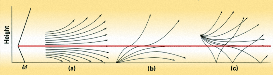
This illustration shows the effects of the Thermal Inversion layer (marked as a red line) on the bending characteristics of VHF-UHF radio waves. The shallow angle signals tend to bend and stay within either the lower or the upper portion around the inversion layer. As a consequence, at times, communication from the ground to somewhere above the inversion layer at long distances might become difficult.
The sub-parts (b) and (c) in the above illustration clarify the above concept further. Although the signals approaching the boundary at shallow angles will not crossover, the higher angle signals will manage to crossover. This phenomenon gives rise to some of the issues that we might face.
- Signals to-and-fro between LEO satellites and earth stations often get drastically degraded during strong Tropospheric ducting conditions. This happens when the satellites are at low angles near the horizon because the signals find it very difficult to cross over to the other side of the inversion boundary.
- Communication between a ground station and an aeronautical asset (aircraft) at a long distance and at a high altitude may become difficult and might get disrupted due to ducting effects. The communication range might get reduced and the SNR might become poor.
- Radar acquisition and detection range might get reduced due to high attenuation of signals penetrating the inversion boundary. The position accuracy of the Radar object might also get compromised due to the bending of Radar signals while penetrating the boundary layer. Furthermore, the Radar noise floor might also get elevated resulting in additional clutter and detection anomalies.
In this article, we have tried to understand the important aspects of atmospheric (Tropospheric) phenomena and their effects on VHF radio communication and beyond. In the next article, we will unravel several other mysteries related to various mechanisms that cause propagation path losses in terrestrial VHF radio communication circuits.


(18 votes, Rating: 5.00) - Please vote the article with your valuable star rating. Thanks! Basu (VU2NSB)
SSN SSNf(10.7) – Real-time Solar Data