

How do Yagi Antennas work?
Perhaps, we all know that a Yagi antenna provides a unidirectional radiation lobe pattern and enhanced forward gain in comparison to a dipole. However, some might ask, what is the unique concept that makes a Yagi antenna tick? What makes it distinctively different from other types of antennas? … Fair question! We will try to examine some of the fundamentals of a Yagi-Uda antenna.
What is a Yagi antenna?
In simple terms, a Yagi antenna is an array of dipoles geometrically arranged in the plane of the primary driven dipole. All the other dipoles of the array barring only one dipole element are not electrically connected to the transmitter. The single dipole which is directly powered by the transmitter is the primary dipole called the driven element. All other electrically unconnected sets of dipoles are called parasitic elements and are geometrically placed in parallel to the driven element at various distances away from the driven element. Hence the Yagi is actually a dipole array. The clever arrangement of actively driving only one dipole while letting the other parasitic dipoles be coupled to the driven element through mutual field coupling is the salient feature of a Yagi antenna. The length of these parasitic elements is almost equal to that of the main driven resonant dipole but they are not exactly equal. Some elements are made a bit longer while the others are made a bit shorter. Hence, essentially, though the parasitic elements are sized to be near resonance, they are not exactly at resonance.

A typical multi-element Yagi antenna
We said before that the more the number of parasitic elements in a Yagi antenna configuration, the greater is the achievable forward gain. Though this is true, we need to bear several limiting factors in mind while designing or accessing a Yagi antenna. Firstly, it becomes impractical to increase the number of parasitic elements beyond a point. This is not merely on account of physical size constraints but also due to the fact that theoretically when we double the number of Yagi antenna elements we get an additional gain of approximately +3dB. Hence, if a 3-element Yagi produces a forward gain of say 12dBi, then a 6-element version will have a gain of 15dBi, a 12-element version will have 18dBi, a 24-element version will yield 21dBi. We notice that the law of diminishing returns starts applying beyond a point. After a point, it becomes difficult to justify the monstrous physical length of the structure which happens due to the size multiplication by a factor x2 required for each 3dB additional gain that we seek.
Another factor to keep in mind is that although a standalone dipole element would also have a finite limited usable bandwidth, the Yagi antenna configuration consisting of multiple dipoles results in a further reduction in the bandwidth in comparison to a simple dipole. The more the number of parasitic elements, the lower is the useful SWR limited bandwidth of the Yagi. A notable factor at this point is to also recognize that compact and short boom Yagi designs will usually have a much lower bandwidth than that of a long boom design where the parasitic elements are more widely spaced. This is true even if they both have the same number of elements… The fact of the matter is, everything good in life comes with a price. There is never a free lunch.
Effect of parasitic elements on the feed-point impedance of a Yagi
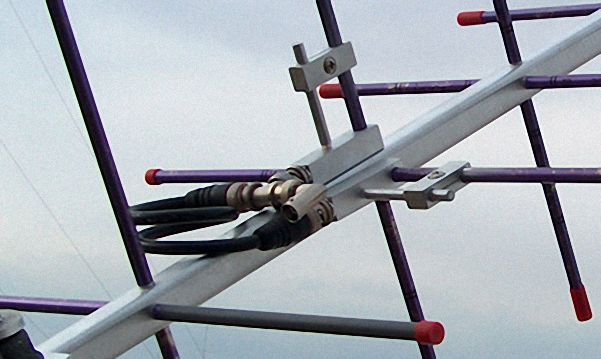
A pair of Gamma Match section on my VHF Crossed Yagi
Depending on the other design objectives, the parasitic element spacing and lengths are so adjusted to achieve far lower feed-point impedances. it is common to find Yagi antennas with a feed-point impedance of either 25-28Ω or 12.5Ω. These values are often preferred by Yagi designers when the Yagi is meant to be a part of a larger stacked antenna array. This makes it convenient to easily design a proper phasing harness for driving the antenna stack. Even the normal standalone Yagi would often have a feed-point impedance of around 25Ω. That is why we so often find Yagi installations using impedance matching methods like a Gamma match to match it to the nominal 50Ω characteristic impedance of common coaxial cables.
Another method often used especially for VHF/UHF compact Yagi designs, is to use a folded dipole driven element instead of a straight dipole. With a straight dipole in a compact yagi design with closely spaced elements, it is fairly common to load the driven dipole enough to achieve a 12-13Ω feed-point impedance. Now, if a folded dipole-driven element were to be used instead, what would happen? The folded dipole has a 300Ω native impedance as against 72Ω for the straight dipole. This is roughly 4 times higher. Hence, a compact yagi whit a straight dipole which might have loaded the driven dipole enough to reduce the impedance from 72Ω to say 12.5Ω would load the Yagi with a folded dipole with the same ratio. In such a case, the 300Ω native impedance of the folded dipole will now get loaded just enough to produce 50Ω feed-point impedance. External impedance matching networks would not be needed anymore. All that one needs is a 1:1 Unun to connect to a 50Ω coax feeder.
Similarly, one might have seen various Yagi antennas, especially on VHF/UHF bands, that have a Quad loop as the driven element instead of a straight dipole that is normally used as a driven element. This type of Yagi is called a Quagi antenna. It derives its name from a Quad and a Yagi. Why do they use a Quagi? Is it that it provides better gain or enhanced performance? No, certainly not… All performance parameters of a Quagi are practically identical to that of a Yagi. Then, why go through all the trouble? Fair question… The answer is that a standalone Quad loop-driven element has approximately 100Ω feed-point impedance. Hence, in an array with several parasitic elements, despite the additional loading of parasitic elements, the reduction in overall feed-point impedance of the Quagi antenna would reduce enough to be close to a typical 50Ω transmission line impedance. consequently, a Quagi will not need elaborate impedance matching networks unlike the Yagi in similar conditions.
How does a Yagi antenna work? How does it produce gain?
Let us see how do Yagi antennas produce forward gain. I will try to keep the narrative simple and intuitive for now and save the rest for a bit later. Before we go further, let us see how the parasitic elements of a Yagi play a role. Since they are electrically isolated from the driven element, how is it that they influence the antenna system? We know that all the parasitic elements are placed in close proximity to the driven element. Hence they are coupled to the driven element through mutual field coupling. All parasitic elements are close enough to lie within the induction field (Raliegh zone) of the driven dipole. If you have missed out on our article explaining the induction field and other zones around an antenna, then please refer to the article on Principles of Radiation to get an insight.
In the induction field region, all conductors achieve a direct coupling to the radiating element through mutual induction. These nearby conductors (parasitic elements in this case) produce a load on the radiating element (driven dipole in this case). As a consequence power is transferred to the parasitic elements from the driven dipole through mutual coupling. The degree and nature of coupling will depend on the distance and the length of the parasitic element w.r.t the radiator. This phenomenon is used to our advantage in a Yagi design, however, in day-to-day scenarios of amateur radio station antennas, this phenomenon may often play a detrimental role. For instance, nearby water pipes, overhead wires, metal in buildings like beams and columns, etc, on account of near field mutual coupling often deteriorate the overall performance of our antenna in terms of efficiency, its radiation lobe pattern, etc.

Phase interference of signals between elements of a Yagi
The above scenario is like having multiple radiating dipoles strategically placed at a proper distance from one another. Due to the separating distance between all these radiating elements, their radiations are out of phase by a certain amount which is proportionate to the physical distance between each other. Their radiations could either constructively or destructively interfere with one another. However, what we want is that the constructive interference should be as high as possible in the forward direction of the Yagi antenna so that they enhance each other to boost the effective radiated power in the forward direction. Similarly, in the reverse direction, towards the back of the Yagi, we want to maximize destructive interference to cancel out the effective radiation.
This is where the cleverest part of the Yagi design comes into play. If we increase the length of a parasitic element beyond its resonant length, then it develops an inductive reactance resulting in a further phase delay of the reradiation from that element. That is how the reflector of the Yagi is made. It is made longer than the driven element. On the other hand, the director(s) of a Yagi is made shorter than the resonant length. This results in a capacitive reactance on the directors which results in the directors further advancing the phase of the reradiated signals. These additional phase shifts offered by the reflector and director(s) work in our favor to achieve signal strength enhancement in the forward direction while suppressing radiation in the backward direction.
Wait a minute… is that all? Nah! … Something seems to be horrendously wrong. What I described in the above paragraph would actually produce enhanced radiation in the backward direction while producing minima in the forward direction. That would be just the opposite of what we want. Oh god! where did we go wrong? … Well, relax, we didn’t get anything wrong. It’s just that, so far, I have not yet mentioned the most important fine point of a Yagi antenna design. Most narratives on the internet and elsewhere are at times a bit fuzzy about the point that we will touch upon now. Our narrative till the previous paragraph, explains the principles of a Yagi provided we ignore to speak about the lobe direction. The fact of the matter is that the Yagi indeed enhances radiation in the forward direction of the directors and not in the backward direction.
Good! So, what would explain the apparent anomaly? Surprisingly, the explanation is rather simple. We must emphasize that all parasitic elements which reradiate including the reflector and the director(s) must be short-circuited in the middle for a Yagi to function. In other words, they must be joined at the center and not be two electrically isolated pieces of 1/2 size elements on either side of the boom. This is very vital. As a consequence of the short-circuiting in the middle, the phase of the current induced in the parasitic elements gets reversed in phase by 180°. Hence, all the phase relationships we discussed so far go through a 180° phase reversal from what we described so far. Therefore, when this phenomenon is applied across the board, and applicable to all parasitic elements of the Yagi, the directions of constructive and destructive interference also get reversed by 180°. Hence, the Yagi radiation lobes do actually indeed get enhanced in the forward direction and not in the reverse direction.
If you want to dig deeper, then read the following section.
OK… So far so good but I want to know more.
Fair enough… Let us start. So as not to make it too complicated, let us take a simple example of a 2-element Yagi with a reflector and a driven element. The explanation can be thereafter extended to scenarios where more elements are added in the form of directors. Without taking more time, let us now straightaway dig into our 2-element Yagi. We will do some simple calculations to not only acquire a better insight into the concept of the Yagi in greater detail but will also compute the forward gain of the Yagi w.r.t a dipole, its signal suppression at the rear, and subsequently deriving at the front-to-back (F/B) ratio of our example Yagi.
![Yagi current phase]() Take a look at the adjasent illustration. It represents a 2-element Yagi antenna. It also shows the phase relationship of currents flowing on both the driven element and the reflector. The typical radiation pattern of this antenna is also displayed for reference.
Take a look at the adjasent illustration. It represents a 2-element Yagi antenna. It also shows the phase relationship of currents flowing on both the driven element and the reflector. The typical radiation pattern of this antenna is also displayed for reference.
The phase of the current on the driven element is 0° which is our phase reference point, while that of the reflector is 140°. Both these values can be confirmed by the phase current color-coded elements and a color code bar on the left. We can see, the reradiation from the reflector will be 140° out of phase w.r.t the driven element. Please also note that this antenna is a compact Yagi design where the physical spacing between the two elements is 1/8λ.
Due to the longer length of the reflector, it appears as a complex load with inductive reactance. Hence it produces a lagging current on it which results in a phase lag. In our example the additional length of the reflector is such that it produces a phase lag of 40°. Since, as mentioned earlier, the reflector is a single conductor length that is short-circuited at the center, it produces a 180° phase reversal of the current. Hence, effectively the 40° phase lag turns into a 40° phase lead when mirrored at 180°. This means that the effective total phase shift of the reflector current w.r.t the driven element will now be 180-40 which is 140°. This is precisely what we see.
Now we come to the most interesting part of our analysis. However, before we proceed further, let us introduce ourselves to the way two vectors are added. This is important because the signals radiated from the driven element as well as the induced reradiation from the reflector are both vectors. Therefore, when we would need to add their magnitudes, we simply cannot add the magnitudes as we normally do in the case of scaler addition. They both have magnitude and phase. Hence, to be able to compute the forward gain, backward gain, and F/B ratio, we will need to add the two radiated signal values using vector addition. Here, in our case, we will only be interested in finding the resultant magnitude of the addition of 2 vectors and not on the resultant phase. Hence, we will restrict ourselves to a single mathematical equation for calculating the resultant magnitude of the addition of two vectors.
Here is the vector addition equation for resultant magnitude…
![Vector add formula]()
Though the magnitude of radiation from the driven element and the reflector will actually be slightly different, for the sake of simplicity, let us assume them to be equal. Let us assign both the vector magnitudes as one (1).
Let us first compute the resultant radiation field strength produced by the Yagi in the forward direction where we expect to achieve some gain. In the forward direction, just barely ahead of the driven element, the radiation vector of the driven element is 1∠0° (magnitude 1 and phase 0°). The Radiation vector from the reflector is 1∠140° (magnitude 1 and 140° angle). Next, let us take into account the physical separation distance between the reflector and the driven element. we noted earlier that it is 1/8λ (0.125λ).
For the radiation from the reflector traveling in the forward direction to reach the driven element where both signal vectors will get vectorially added, the reflector radiation has to travel an extra 1/8λ distance. Therefore, by the time the reflector's radiation vector reaches the front of the Yagi, the phase of the radiating vector of the driven element would have changed. How much will that change be? It will be 0.125x360 (where 360° corresponds to 1λ). Don't forget, the travel distance between the reflector and the driven element is 1/8λ (0.125λ) The result of 0.125x360 = 45°. This means the net difference between the phase of the reflector radiation vector (140°) arriving at the driven element and the phase of the driven element field vector at the time when the vector from the reflector arrives will be 140+45 = 95°.
Let us now apply the vector addition equation and find out how much gain enhancement we get if any. Since we assumed that both vector magnitudes are unity (1), the variable "a" and "b" applied to the equation will both be one (1). The angle θ in our equation will be 95°.
The result of the above calculation is 1.35118. This is the magnitude of expected forward gain. Let us now convert this magnitude into dB. Since the vectors that were added were field vectors and not power vectors, we would compute the dB as 20xlog(1.35118) = 2.614. This means that our 2-element Yagi antenna will produce about 2.6dB gain enhancement in the forward direction. This is very much in line with what we would expect in reality.
So far so good. Now, let us examine the field strength at the back of the Yagi antenna array. Following a similar method, as we did for the forward direction, we will try to see what would happen at a point that is just behind the reflector. This time, it is the radiation field of the driven element which is at 0° phase will have to travel towards the back across 1/8λ distance to reach the reflector of the array. While this happens, the energy field radiated from the reflector would have changed its phase by 0.125x360 = 45°. Hence, the phase of the reflector field which was initially 140° will be 140+45 = 185°. Therefore, the phase relationship (difference) between the signal field from the driven element and the reflector will be 185+0 = 185° at the time when the radiation from the driven element (traveling backward) reaches the reflector. The resultant composite field strength at the back of the Yagi will be a vector addition of the two signal vectors as computed by our vector addition equation. This calculates to a value of 0.08723. The equivalent value in dB notation will be 20xlog(0.08723) = -21.186. Hence, the backward signal field is attenuated by about -21.2dB.
If we were to apply both the above findings, we find that the Front-to-Back (F/B) ratio of our Yagi antenna is 21.2 + 2.6 = 23.8dB. Isn't it remarkable? That's all for now... We have successfully calculated a few vital performance metrics for our example Yagi and established that it indeed has a positive gain in the forward direction while attenuating strongly in the backward direction.
To conclude our discussion, here is the summary of our calculations for our 2-element Yagi antenna...
Fair enough… Let us start. So as not to make it too complicated, let us take a simple example of a 2-element Yagi with a reflector and a driven element. The explanation can be thereafter extended to scenarios where more elements are added in the form of directors. Without taking more time, let us now straightaway dig into our 2-element Yagi. We will do some simple calculations to not only acquire a better insight into the concept of the Yagi in greater detail but will also compute the forward gain of the Yagi w.r.t a dipole, its signal suppression at the rear, and subsequently deriving at the front-to-back (F/B) ratio of our example Yagi.

Phase relationship of currents on both elements of a 2-el Yagi
The phase of the current on the driven element is 0° which is our phase reference point, while that of the reflector is 140°. Both these values can be confirmed by the phase current color-coded elements and a color code bar on the left. We can see, the reradiation from the reflector will be 140° out of phase w.r.t the driven element. Please also note that this antenna is a compact Yagi design where the physical spacing between the two elements is 1/8λ.
Due to the longer length of the reflector, it appears as a complex load with inductive reactance. Hence it produces a lagging current on it which results in a phase lag. In our example the additional length of the reflector is such that it produces a phase lag of 40°. Since, as mentioned earlier, the reflector is a single conductor length that is short-circuited at the center, it produces a 180° phase reversal of the current. Hence, effectively the 40° phase lag turns into a 40° phase lead when mirrored at 180°. This means that the effective total phase shift of the reflector current w.r.t the driven element will now be 180-40 which is 140°. This is precisely what we see.
Now we come to the most interesting part of our analysis. However, before we proceed further, let us introduce ourselves to the way two vectors are added. This is important because the signals radiated from the driven element as well as the induced reradiation from the reflector are both vectors. Therefore, when we would need to add their magnitudes, we simply cannot add the magnitudes as we normally do in the case of scaler addition. They both have magnitude and phase. Hence, to be able to compute the forward gain, backward gain, and F/B ratio, we will need to add the two radiated signal values using vector addition. Here, in our case, we will only be interested in finding the resultant magnitude of the addition of 2 vectors and not on the resultant phase. Hence, we will restrict ourselves to a single mathematical equation for calculating the resultant magnitude of the addition of two vectors.
Here is the vector addition equation for resultant magnitude…

Though the magnitude of radiation from the driven element and the reflector will actually be slightly different, for the sake of simplicity, let us assume them to be equal. Let us assign both the vector magnitudes as one (1).
Let us first compute the resultant radiation field strength produced by the Yagi in the forward direction where we expect to achieve some gain. In the forward direction, just barely ahead of the driven element, the radiation vector of the driven element is 1∠0° (magnitude 1 and phase 0°). The Radiation vector from the reflector is 1∠140° (magnitude 1 and 140° angle). Next, let us take into account the physical separation distance between the reflector and the driven element. we noted earlier that it is 1/8λ (0.125λ).
For the radiation from the reflector traveling in the forward direction to reach the driven element where both signal vectors will get vectorially added, the reflector radiation has to travel an extra 1/8λ distance. Therefore, by the time the reflector's radiation vector reaches the front of the Yagi, the phase of the radiating vector of the driven element would have changed. How much will that change be? It will be 0.125x360 (where 360° corresponds to 1λ). Don't forget, the travel distance between the reflector and the driven element is 1/8λ (0.125λ) The result of 0.125x360 = 45°. This means the net difference between the phase of the reflector radiation vector (140°) arriving at the driven element and the phase of the driven element field vector at the time when the vector from the reflector arrives will be 140+45 = 95°.
Let us now apply the vector addition equation and find out how much gain enhancement we get if any. Since we assumed that both vector magnitudes are unity (1), the variable "a" and "b" applied to the equation will both be one (1). The angle θ in our equation will be 95°.
The result of the above calculation is 1.35118. This is the magnitude of expected forward gain. Let us now convert this magnitude into dB. Since the vectors that were added were field vectors and not power vectors, we would compute the dB as 20xlog(1.35118) = 2.614. This means that our 2-element Yagi antenna will produce about 2.6dB gain enhancement in the forward direction. This is very much in line with what we would expect in reality.
So far so good. Now, let us examine the field strength at the back of the Yagi antenna array. Following a similar method, as we did for the forward direction, we will try to see what would happen at a point that is just behind the reflector. This time, it is the radiation field of the driven element which is at 0° phase will have to travel towards the back across 1/8λ distance to reach the reflector of the array. While this happens, the energy field radiated from the reflector would have changed its phase by 0.125x360 = 45°. Hence, the phase of the reflector field which was initially 140° will be 140+45 = 185°. Therefore, the phase relationship (difference) between the signal field from the driven element and the reflector will be 185+0 = 185° at the time when the radiation from the driven element (traveling backward) reaches the reflector. The resultant composite field strength at the back of the Yagi will be a vector addition of the two signal vectors as computed by our vector addition equation. This calculates to a value of 0.08723. The equivalent value in dB notation will be 20xlog(0.08723) = -21.186. Hence, the backward signal field is attenuated by about -21.2dB.
If we were to apply both the above findings, we find that the Front-to-Back (F/B) ratio of our Yagi antenna is 21.2 + 2.6 = 23.8dB. Isn't it remarkable? That's all for now... We have successfully calculated a few vital performance metrics for our example Yagi and established that it indeed has a positive gain in the forward direction while attenuating strongly in the backward direction.
To conclude our discussion, here is the summary of our calculations for our 2-element Yagi antenna...
- The forward gain enhancement over a dipole gain is 2.16dB.
- The backward attenuation is -21.2dB.
- The F/B ratio is 23.8dB.
- In free-space where a typical dipole has 2.15dBi gain, the forward gain of our Yagi will be 2.15+2.61 = 4.76dBi, the backside attenuation will be 2.15+(-21.2) = -19.05dB while F/B ratio remains 23.8dB.
- In a practical HF installation scenario above ground, where about 8dBi gain of a standalone dipole elements might be expected, the forward gain will be 8+2.61 = 10.61dBi, the backside attenuation will be 8+(-21.2) = -13.2dB while F/B ratio remains 23.8dB.
I hope you enjoyed reading the article. Perhaps some readers might have gained a better insight into the finer yet lesser-known facts about the Yagi-Uda antenna that we all admire and use quite often.


(21 votes, Rating: 5.00) - Please vote the article with your valuable star rating. Thanks! Basu (VU2NSB)

Ham Rig Reviews Coming Soon
SSN SSNf(10.7) – Real-time Solar Data


