Radio propagation forecasting and assessment
When we speak of forecasting and assessment with reference to HF radio, they often mean two different things. Assessing HF radio propagation conditions to plan radio communication has been in vogue for a long time. Various methods have been used by both professionals as well as radio amateurs. One of the cornerstones of long-range HF propagation assessment has been the time-tested method of using radiofrequency beacons. On the other hand, propagation forecasting is more a science-based on the projections made using mathematical models of the Solar activity, Ionospheric models, and extrapolation from historical measurements. These methods have been refined and combined scientifically to make fairly good HF band propagation forecasts.
In this article, we will examine some of these methods to be able to use the information to our advantage for day-to-day radio communication. Our narrative will focus on HF radio propagation.
The Beacon System for Radio Propagation Assesment
Since the good old days, radiofrequency beacons have served as useful and friendly tools for amateur radio operators around the world. Essentially beacons are low or medium-power radio frequency transmitters set up at various locations around the world across continents. They are designed to run continuously in an autonomous mode. Typically, these beacons are designed to repetitively transmit a short CW (morse code) sequence. Normally, the transmission comprises a designated callsign that identifies the beacon thus allowing the receiving station to know its geographic location.
A typical received CW radio beacon transmission as shown on a waterfall display of an HF transceiver.
The best part about using beacons for radio propagation assessment is that unlike forecasts based on mathematical models, it is real-time and truly as it prevails. Therefore, drawing inferences based on beacons can never be incorrect. Since HF radio propagation through Skywave skip propagation rarely alters on a kilometer to kilometer basis, the reception of a beacon signal from the DX land usually indicates that there could be possibilities of establishing contacts with other radio stations around the region of the beacon. The area of available propagation coverage would at least be several hundreds of square kilometers around the beacon location. Quite often the indicated radio propagation opening may extend to several tens of thousand kilometers, perhaps coving the entire county including several adjoining countries too.
Quite often, a distant beacon can be copied with sufficient signal strength for an extended duration of time for several hours with significant alteration in signal strength. This is indicative of robust and long-term radio propagation opening on that band. By motoring various beacons from different parts of the world on a particular band, an experienced radio amateur can effectively gauge the nature of radio propagation opening that prevails at that time across the entire global canvas. Moreover, a radio operator who might monitor various geographically spaced out beacons on several bands is usually in a position to assess the probability of global openings on different bands and also the pattern of the transition of these openings from one band to another.
Another interesting fact about radio propagation assessment using beacons is that due to the nature of the ionospheric behavior, it is quite probable that the observations made on a particular day will hold good for the next few days. Barring conditions of sudden solar activity like a CME, etc, the chances are good that the propagation conditions would nearly repeat themselves the next day and so on. Remember that our ionosphere has considerable inertia and does not alter its characteristics drastically on a day-to-day basis. Neither does the declination of the sun alter rapidly. Hence, the ionospheric behavior also nearly repeats itself the next day, only to change gradually over the weeks. Not only can the basic radio propagation prospects be determined by monitoring beacon transmissions but several other important inferences can also be drawn fairly well. For instance, an experienced station operator may be able to determine communication prospects based on different modes of communication. S-meter reading of the CW beacon can be used to determine whether the radio propagation conditions are good enough to allow a sustainable SSB radio-telephony QSO or if the signal strength is only good enough for lower bandwidth modes like PSK31 or FT8 and so on so forth.
The modern NCDXF(IARU) Beacon Network

Animated display of the typical switching sequence of NCDXF beacon set from one to another on an HF band. (Note: Inter-beacon switching time has been made quicker in the animation)
The NCDXF beacon network uses a time-division multiplexing paradigm. By monitoring a single beacon frequency on any band, the amateur radio operator can gather enough information within a couple of minutes regarding the prevailing propagation prospects around the entire world. The transmission on the beacon frequency cyclically switches from one beacon to another covering all the 18 beacons one after another. This pattern of transmission continuously repeats itself. Each beacon transmits for a duration of 10 seconds before switching over to the next beacon located at another place.
Each transmission from any beacon comprises of its callsign in CW at 22 words per minute and 100W EIRP TX power into omnidirectional antennas. This is followed by 4 distinctive short-length carrier transmissions of one-second duration each in the form of 4 consecutive dashes.
Now, we come to the most interesting part that makes this beacon system so remarkable. The 4 dashes that are transmitted after the callsign are not transmitted at a constant power level. These dashes follow a graded power sequence. The first dash after the callsign is at 100W, whereas the following 3 dashes are transmitted at 10W, 1W, and 100mW levels respectively. Hence the variation of the signal power is 10dB between two consecutive dashes. This covers a total dynamic range of 40dB. It is this attribute that makes these beacons so awesome. This allows the station operator at the receiving end not only to make a subjective assessment but allows him to make a rough quantitative assessment of prevailing propagation.
The cyclic sequence of beacons transmitting on a band is from 18 distinctive geographic locations. These locations are as under…
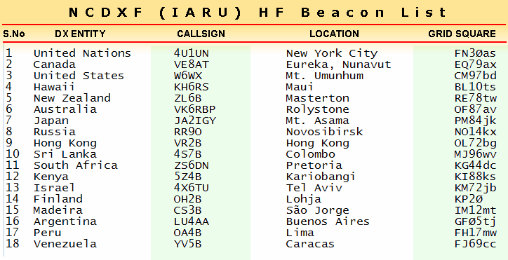
List of 18 NCDXF (IARU) beacons that run in time-division multiplex mode on each DX band with 10 second time-slots and repeat the cycle every 3 minutes.
Before we shift focus from the beacon-based propagation assessment to the mathematical model based forecasting paradigms, let us quickly recap the important features of the NCDXF(IARU) Beacon system…
- 18 CW beacons broadly cover the entire world using strategic locations.
- The system uses multiplexing (TDM) to sequentially cover all locations.
- NCDXF beacon system covers all five DX bands, the 20-17-15-12-10m
- Each beacon transmission on any band lasts for 10 seconds.
- All the 18 transmission slots are covered in 18×10=180 seconds (3 minutes).
- The cyclic repetition of the transmission cycle occurs every 3 minutes on any band.
- All 5 HF beacon bands are covered offsetting transmission slots within the 3-minute cycle.
- The handover of transmission or switching of a band from one beacon to the next is synchronized globally using an accurate atomic clock.
- On each band, only one frequency is needed to be monitored for a minimum period of 3 minutes to asses the actual prevailing propagation scenario in real-time across the world.
- Four-step graded power emission (100-10-1-0.1W) during each beacon transmission provides greater depth to the assessment of the propagation conditions.
- Last but not the least, for all those who lack CW skills to identify beacon callsigns, several free software utilities are available that identify beacons in real-time while they transmit.
Radio Propagation Forecast Models and Tools (VOACAP, etc.)
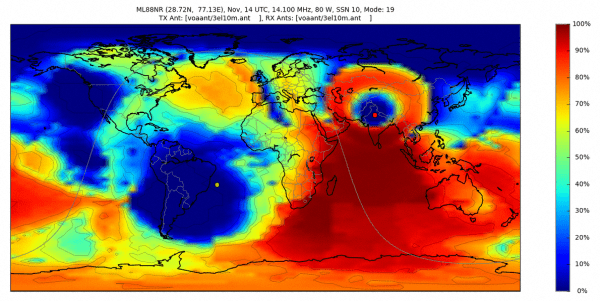
An example of a map rendition of propagation forecast on 20m band from VU2NSB QTH in New Delhi, India during Nov’2019 at 14:00 UTC on 20m band.
Beacon-based assessment paints the scenario for us in true colors, whereas the forecasting methods provide us with a probable scenario with no guarantees. Beacons automatically account for, station antenna performances, efficiency, general capabilities, etc in their reporting, whereas forecasting has to be done by providing manual inputs to the model. This is where many people make wrong judgments. Moreover, forecasting of any kind is entirely based on statistical probability, whereas, beacon-based assessment is real and actual as it prevails.
Having said that, the propagation forecasting model-based systems too have many plus points that are very attractive. They allow for better presentation formats which include charts and graphical rendition of forecasts. They also present a more spatial resolution in comparison to the beacon networks. The beacons are placed at widely spread locations and are limited in number. Hence, the beacons require a far better understanding of geography as well as general radio wave propagation to be able to draw meaningful inferences of propagation conditions prevailing further away from the beacon locations, whereas, in the case of forecasting systems, all this work is done by the computers.
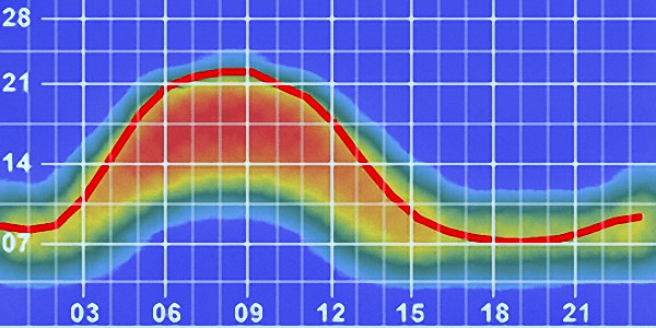
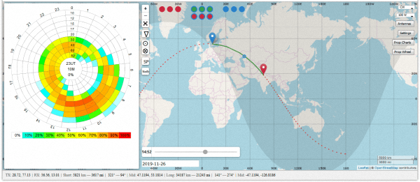
Point-to-point HF propagation forecast between two locations on earth. The forecast covers a 24 Hr. cycle and depicts band opening in color-coded format. MUF is shown as solid red line curve. (X-axis: Time, Y-axis: Frequency)
However, one must never lose sight of the fact that radio propagation forecasts are usually approximations and not absolute. The radio propagation forecasting models require several input parameters that are needed to drive the forecast engine. Quite often, many of these parameters are not as accurate as what one might like them to be. Moreover, none of the common forecast models account for short-term, spurious, or anomalous and secondary effects of mother nature that may affect the propagation conditions. The results of these forecasts are generally statistical information that is often averaged over days of what might be expected. Nevertheless, they provide quite useful information to help us understand expected propagation trends that we might encounter in the coming days.
The bottom line is that the beacon-based networks present the pudding, while the forecast models present us with the recipe of the pudding and tell us how it might probably taste if it were to be there.
After having truthfully examined the merits and limitations of radio propagation forecasting systems in general, let us now take a look at typical models that are available to the amateur radio community for HF radio propagation forecasting.
VOACAP HF Radio Propagation Forecast Software
The abbreviation VOACAP stands for Voice Of America Coverage Analysis Program. This has a history of development that started off with efforts of the U.S. Military for forecasting Ionospheric behavior. They originally developed a DOS software called IONCAP (Ionospheric Communication Analysis Prediction). Thereafter further funding was required to continue development. Voice of America (VOA) chipped in to push further development. This resulted in branching off to what came to be known as VOACAP. Around the same time, the Institute of Telecommunication Science (ITS) continued to further develop IONCAP thus creating a separate software branch off that they called ICEPAC (Ionospheric Communications Enhanced Profile Analysis and Circuit Prediction). ICEPAC accounted for additional parameters that could be more useful for modeling Aurora-driven conditions near the polar regions.
So, we had the original IONCAP, the ITS lead ICEPAC and VOA sponsored VOACAP that was also supported by Naval Research Laboratory in the U.S.A… All of these programs continued to be developed. However, we will focus on VOACAP since it happens to be the one that has developed into a form that is broadly most suitable for amateur radio applications.
VOACAP Online service to provide HF Skywave propagation forecasts.
Now, as we see, the focus of VOACAP was essentially on analyzing radio broadcast coverage for shortwave commercial broadcast stations. Their requirements were quite different from those of radio amateurs. Before setting up new transmitters or planning the expansion of service coverage, the broadcast companies were interested in knowing the reliable coverage that they could possibly obtain throughout the year to plan region-wise targeted broadcasting of their programs. They also needed to plan reliable overseas broadcast coverage. Therefore, the emphasis of VOACAP was not to find HF band radio propagation opening variations on a day-to-day basis. This was the least of their concern. They actually needed to generate scientifically analyzed statistical data to be able to forecast the reliability of broadcast coverage across the target region.
Therefore, by default, VOACAP presents the statistical probability of communication reliability in percentage terms. This is based on a reference level of acceptable signal-to-noise ratio (SNR) that would be required for a sustainable radio signal received at the remote location. The reliability percentage also factors in typical levels of signal fading that could be encountered. Based on these and other variables, by default, VOACAP forecasting software works as under…
Limitations and Strengths of VOACAP from Amateur Radio Perspective.
VOACAP HF radio propagation forecasting service is available for free use by radio amateurs on the internet at VOACAP Online. Please note that there are at least two other versions of this service with different URLs that are also available which are primarily tailored for broadcast and maritime station use. Do not choose the wrong version and avoid confusion between them.
Before we begin to examine some of the practical limitations of VOACAP, let me categorically state that it is a marvelous piece of software. It is very well-conceived and nicely designed. Whatever perceived limitations that we might discuss below may actually not strictly be its limitations at all. We often tend to have over expectations from something that it was not originally even intended to do. That applies to VOACAP too. I have come across many people who expect VOACAP to provide a gospel truth in its forecasts and they expect its results to perfectly match the prevailing real-world propagation scenario in real-time… That’s not what VOACAP was ever intended to do. VOACAP is supposed to provide us the larger picture to allow us to plan communication prospects across the world, between any locations, on any HF band, and during any time segment. It does this job pretty well provided the user knows how to choose and fine-tune various input variables judiciously before running a forecast on VOACAP.
A Quick Checklist of VOACAP Facts & Myths
- VOACAP forecasts a one-month average of the expected reliability of signal transmission to be available at a remote location in percentage terms.
- Percentage Reliability implies that the expected percent of the days in a month when propagation is expected to be favorable.
- To arrive at the forecast, by default, VOACAP uses a monthly predicted average of SSN as input to the forecast engine.
- VOACAP may use either CCIR-66 or URSI ionospheric data model to compute forecasts. (More on this later in the article)
- VOACAP does not account for short-term variations in ionospheric behavior that may regularly be caused on account of solar emission variations, CME, solar storms, etc.
- Therefore VOACAP does not account for day-to-day ionospheric disturbances, magnetic disturbances or anomalies, A-index, K-index, auroral effects, variation in energy densities of solar proton flux, etc.
- VOACAP does not take into account the ground wave propagation or any other propagation modes except for ionospheric Skywave propagation.
- However, VOACAP does account for diurnal variations as the earth spins on its axis.
- VOACAP also accounts for the day-to-day variations due to seasonal shifts attributed to the declination of the earth resulting in a gradual change in the sub-solar latitude of the Sun’s footprint.
- Although the default forecast projection format is link reliability, VOACAP also projects expected signal power density (SDBW), noise power density (NDBW), Maximum usable frequency (MUF), signal-to-Noise ratio (SNR), etc… However, all these projections are based on the monthly average of predicted solar data metrics affecting the ionosphere and are not real-time conditions.
Despite various limitations cited above, the VOACAP Radio propagation forecast system driven by the ITSHFBC core engine is a very useful tool that provides great insight into the way HF ionospheric Skywave radio propagation works. It also provides us with a fairly good average projection of the nature of radio propagation to expect on the HF bands for the medium and long-range communication circuits.

A Typical propagation forecast chart generated by VOACAP.
For the experienced user who might have a sufficient understanding of the finer nuances of radio propagation, VOACAP also allows overriding its default settings and lets one enter custom an SSN value, select man-made noise-floor level, and opt for a different minimum radiation takeoff angle (TOA) of selected antennas.
VOACAP Online is a nice radio propagation forecasting system adapted for amateur radio use. However, one must avoid falling into the trap of over-reading or over-relying on its forecasts. Many ham operators I know have often tried to compare the real on-band results with the forecast made by VOACAP. They all ended up being quite taken aback and often grumbled about something being wrong. One must always keep in mind the inherent limitations of any tool while using it and only draw considered conclusions based on the hard facts.
What are CCIR and URSI Ionospheric Dataset Models?
As I said before, let me emphasize once again that HF ionospheric Skywave propagation forecasting methods used by VOACAP are purely based on historical statistical data that were recorded and collated over many years in the past. VOACAP is primarily dependent on these statistical datasets. The two prominent datasets that are available are the CCIR-66 data collected by ITU and the URSI data collected by Consultative Committee for International Radio (CCIR) of ITU, and Union Radio Scientifique Internationale (URSI) respectively.
The CCIR dataset is also called CCIR-66 since it was formally presented in 1966. URSI dataset is relatively more recent. Both these datasets consist of Ionograms (obtained by radio sounding of Ionosphere). The Ionogram data for foF2, foF1, foE, and foEs were measured from various geographic locations around the world over many years covering entire 11-year solar cycles on an hourly basis. All this data was compiled into datasets.
CCIR exercise was conducted much earlier and it had fewer participating radio sounding stations in the program. The emphasis of measurement was more on the northern hemisphere locations with few and scantly spread ionosonde stations in the southern hemisphere. All ionospheric sounding was done over land mass and nothing was recorded over the oceans. The URSI program later conducted a similar exercise with a far higher ionosonde station density around the world. There were approximately 45000 ionosonde locations in the URSI program.
Since the cyclic behavior of the ionosphere is more-or-less similar and repetitive over various cycles of physical phenomena, it is assumed that the resultant behavior of propagation will also be similar during the current time. This is largely true and hence we manage to arrive at a reasonably good forecast for the current-day scenario.
There is another important approximation that both CCIR, as well as URSI based forecast, need to make. Since neither of the two datasets has a high enough ionosonde location density, the expected ionospheric parameters for any specific geographic location have to be made by interpolation of the data available in the datasets. Similarly, since the recorded data has a frequency of one hour, a time interpolation also needs to be done between two adjacent sets of data.
Both CCIR and URSI data are used by various forecasting programs, the URSI data provides a slight advantage. due to the higher number of recording stations used URSI provides a better location density. It is relatively newer and hence it provides more current data. The SSN range for effective forecasting is larger with URSI dataset.
As the years go by, the recorded data begins to deviate progressively from reality. However, it is not yet of any significant concern and both CCIR and URSI data are holding good. The progressive tilt of the earth’s magnetic axis, the variation of magnetosphere orientation, change in average higher atmospheric composition, etc are some of the factors contributing to the progressive deviation from the recorded ionograms. However, we need not worry about these factors because the rate of change is minuscule. I am sure, by the time it becomes necessary, we will have newer recorded ionogram data available to us.


(16 votes, Rating: 5.00) - Please vote the article with your valuable star rating. Thanks! Basu (VU2NSB)
SSN SSNf(10.7) – Real-time Solar Data