VHF/UHF & Free Space propagation

Authored by: Basu (VU2NSB) on November 10, 2019.

VHF/UHF & Free Space Propagation – A primer

Radio wave propagation across the entire spectrum including VHF, UHF, and microwave primarily depends on the principles of Free Space propagation. As the radio waves propagate, they are subsequently acted upon by several other physical phenomena like reflection, refraction, diffraction, absorption, etc to modify their net behavior. It is therefore important to get a fair insight into the basic aspects of Free Space propagation. To brush up the above concepts, please check out our article on Fundamentals of Radio Propagation.

In the case of VHF/UHF communication that is nowadays commonly trending amongst radio amateurs, quite often most of these modifier effects rarely come into play. The reason being that over the last 30 years or so, a large section of radio amateurs conduct VHF/UHF communication either on short-distance local point-to-point circuits or use repeaters which are at times trunked using hybrid methods like the internet based Echolink or similar platforms. Moreover, the general trend is to use FM radios. This makes propagation on these bands rather mundane and elementary and one is deprived of experiencing the finer nuances that could show up while pursuing DX on VHF and UHF.

VHF/UHF terrestrial radio DXing which at one time was quite prevalent is now perhaps a dying art. The modes like SSB, CW, Amateur Television (ATV) are not so common anymore. Having said that, I would like to state that VHF/UHF DXing is a very exciting aspect of amateur radio communication. When we speak of DXing, we certainly do not mean the long distances that are possible to cover on HF, thanks to the lack of ionospheric propagation on the VHF/UHF bands but communication ranges spanning over several hundred kilometers are often possible.

Basic VHF/UHF propagation methods in general use
In the case of the usual urban and suburban radio communication on these bands using either handheld transceiver (HT) or base station rigs with FM modulation, a large amount of traffic is routed via repeaters that are set up at strategic locations. The rest of the traffic is simplex using either fix station or mobile radio equipment.

Under such scenarios, other than Line-of-Sight (LOS) direct wave propagation, a few other physical effects also play up to either enhance or more often adversely affect communication. These are typically the presence of buildings in the city as well as the nearby geographic entities like hills and valleys. For instance, a cluster of buildings, especially the modern structures made of steel and concrete quite often adversely affect VHF/UHF communication coverage, They absorb RF energy and act as nearly opaque barriers to the line of propagation. However, on a few occasions, these structures may also act as reflectors and enhance signals in certain favored directions.

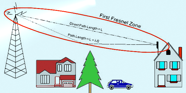
A typical First Fresnel Zone region between two VHF stations

More importantly, perhaps there is another phenomenon that always comes into play in all forms of terrestrial radio communication, yet not duly appreciated by most people, is the effect of Fresnel Zone. In fact, the first Fresnel Zone clearance is vital to establish a point-to-point LOS contact. The Fresnel Zone is an ellipsoidal barrel-shaped region between the antennas at point A and point B of a radio circuit.

To get a greater insight into the concepts of Fresnel Zone, check out this article on Ground wave propagation where we explain it in more detail.

There are multiple Fresnel Zone regions but it is important that the First Fresnel Zone in its entirety must be clear of any obstructions within its barrel-shaped region, or else, communication breakdown might occur. It is not only important for the direct ray path between points to be clear but the entire first Fresnel Zone region must have no obstructions. VHF/UHF and microwave terrestrial communication circuits must take this factor into account to establish reliable communication. Hence, the height of the antennas above ground becomes a very important factor. This is primarily the reason why operators on the ground with hand-held TXRs rarely achieve long-range communication capabilities… More on this important aspect later in a separate article.

The net effect of various factors on urban terrestrial VHF/UHF communication is a mixed bag. Signal ducting along streets surrounded by rows of buildings may often enhance RF signal strength along the street. Corners of buildings may cause knife-edge diffraction to allow signal illumination around a bend. Multi-path propagation on account of reflection from the various structures may often lead to signal fading. This is quite predominant in the case of vehicle-mounted mobile communication that could result in a rapid change in signal strength resulting in fading and flutter.

Terrestrial DXing on the VHF/UHF bands
DXing on VHF/UHF bands is an interesting activity but unfortunately, there aren’t too many DX operators on these bands. Usually, CW and SSB with either voice modulation or narrow-band digital modes are used to establish DX contacts. Unlike the more popular FM mode (either directly or through repeaters) that typically use vertical polarization for communication, the DX operations on VHF/UHF bands are typically conducted with horizontally polarized antennas. Although the polarization compatibility of antennas is inconsequential for HF band DX, it is vital to have identical antenna polarization for terrestrial VHF/UHF DX circuits. Incompatible polarization can practically lead to 20-30dB additional circuit loss and hence ruin the possibility of establishing DX contacts.

Illustration depicting the concept of Meteor Scatter mode

Usually, we find that DXers on these bands use high gain horizontally polarized antennas and stacked arrays. It is quite common to find serious VHF/UHF DX operators using large rotatable Yagi, Quagi, Cubical Quad, or stacked arrays deployed at good height above ground on towers. They invariably use low loss transmission lines and often have mast-head pre-amplifiers at the antenna for receiving purpose. With a setup of this kind, the real fun begins.

It is not only that DX operators leverage the antenna height above ground to reach out further beyond the horizon, but they also use other naturally occurring phenomena to greatly enhance DX coverage. As and when these natural physical phenomena occur on account of atmospheric processes, long-range VHF/UHF terrestrial communication possibilities present exciting prospects.

The most prominent atmospheric phenomena that play up from time to time are tropospheric super-refraction, tropospheric ducting, troposcatter, etc. A couple of ionospheric effects also often manifest themselves to enhance the VHF/UHF communication range. These include the Sporadic-E, meteor scatter, etc, and a few other geographical region-specific phenomena like trans-equatorial propagation due to clumping of electron clouds on both sides of the equator formed by a phenomenon called the Equatorial Electrojet.

All the above phenomena are relatively sporadic in nature, however, they manifest themselves often enough to make them exciting and useful for amateur radio communication. The occurrence of most of these phenomena is dependent on the time of day, the seasons, the warm and cold air layer profile of the lower tropospheric region, the position of the sun vis-a-vis the equator, etc. We will dwell thoroughly into all these phenomena individually through dedicated articles under this section of our website.

6m Band – This is often called the magic band by radio amateurs though there is nothing magical about it. Every nuance of propagation behavior on the 6m band can be explained by well-established scientific phenomena. The beauty of this band is that being at the cusp of the HF and VHF bands, it inherits some of its behavior from both the HF and the VHF bands. Under moderate to high SSN conditions the F2 layer as well as the E-layer propagation occur from time to time over preferred directions. It also works with Sporadic-E, meteor-scatter, atmospheric super-refraction, and tropospheric ducting. 6m band DXers find these propagation methods quite attractive which at times may even yield inter-continental radio contacts.
2m band – This band falls in the middle of the VHF spectrum and is ideally suited for frequent DX using almost all the modes available to the 6m band plus the manifestation of trans-equatorial propagation mode across the equator that might cover DX distances in the order of 6000-8000 Km.
70cm band – Most of the propagation methods cited above are also applicable to this band, however, the probability of robust and reliable Sporadic-E as well as Trans-equatorial openings get significantly reduced due to the lack of sufficient ionization density required at these frequencies. On the other hand, the tropospheric scatter mode becomes more frequently available due to the reduction in wavelength.
23cm and beyond – Many of the above-cited modes of communication begin to become less relevant as we increase the operating frequency, however, the tropospheric scatter becomes more predominant. Atmospheric absorption due to the presence of various gases, dust particles, raindrops, etc tends to increasingly accentuate attenuation. The buildings, architectural artifacts, and natural geographic topological entities start affecting propagation even further. The foliage comprising of trees, plants, etc also contributes to signal attenuation through absorption. By and large, these bands are more suitable for classic point-to-point Line-of-sight (LOS) communication.

Let us now take a brief look into the underlying concept of Free-space propagation. It is the basic building block and the foundation of all modes of propagation. A reasonable understanding of Free space propagation is vital to appreciate the effects of various propagation phenomena that we will subsequently cover in many of our website articles.

Free Space Propagation

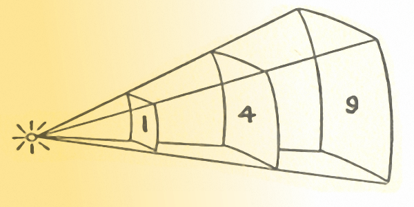
Progressive beam spreading of radio waves during free-space propagation

Let me start by mentioning that although the Free Space propagation mode is very significant while dealing with VHF, UHF and Microwave propagation, generally on its own, it is rather an inconsequential mode for HF terrestrial propagation. However, we will dwell upon several very important fundamental concepts while discussing Free Space propagation. This will be very handy when we eventually dig into other relevant HF propagation modes later through a number of articles on our website. Some of these important concepts are Inverse Square Law, Power Flux Density, E-Field, H-Field, Antenna Aperture, Path Losses, etc.

We have mentioned Free Space Propagation earlier in the article. For all who have a background in science at the school level, the concept should be easy to follow. It is quite intuitive. Just like the light that spreads around in all directions and the intensity of illumination becomes weaker as we move away from the light source, the EM waves (radio waves) also behave in a similar manner. The fact of the matter is that both light and radio waves are EM waves. They are fundamentally the same animal. The only difference between the two is their frequency or wavelength. Radio waves have a much lower frequency (longer wavelength) whereas light waves have extremely high frequency (very short wavelength). Just as a good antenna designed for the specific radio frequency band efficiently picks up radio signals, the retina in a human eye is designed by nature to respond to the frequency band of light and is essentially an antenna at the frequency of the light wave.

Radiation from Isotropic Source

Illustrative depiction of Inverse Square law of propagation

If light were to be emitted from a small light source uniformly in all directions in a three dimensional (3D) space it will spread out with equal brightness and intensity in all directions. Such a light source that emits equally all around in 3D space is called an Isotropic Source. If there was a large globe-shaped lampshade made of translucent (frosted) glass with an isotropic electric bulb at the center, we will notice that the brightness at any point on the surface of the lampshade is equal.

If the diameter or the size of the lampshade is very big we find the glow on the surface of the frosted glass will be less compared to a lampshade of a smaller diameter. The larger the diameter, the surface glow will be less bright. In other words, the longer the distance of the illuminated surface from the point of the light source, the intensity of illumination will be weaker.

The next vital question is how much weaker does the intensity of illumination becomes as we move further and further away from the light source? Is it inversely proportionate to the distance? The answer is no. It does not change or reduce linearly with the distance but in accordance with the square of the distance. Therefore if the distance becomes twice then the intensity becomes one-fourth, if the distance becomes three times then the intensity is one-ninth, and so on so forth.

This is exactly how radio waves also behave. We can replace the light source with a radio transmitter and an isotropic antenna that radiates uniformly in 3D. Since we cannot see the radio wave intensity with our eyes, we may now remove the globe-shaped lampshade and place a radio wave sensor (antenna) at a distance where the lampshade surface was. Hence we have exactly similar situations using radio signals as we had with light.

For those who might like to dig a bit deeper, I would suggest that you should continue to read on. I will try to present some of the very basic, yet important concepts with the aid of elementary mathematics. These concepts will help in acquiring a better understanding of some of the fundaments. Please read on…

Power Flux Density
The surface area of the spherical lampshade or a virtual spherical surface if we consider radio waves can be calculated by the following formula.

A = 4pi D^2

If we assume the power of the transmitter (Isotropic source) is Pt, then the effective illumination intensity (power distribution per unit area of the spherical surface) will have received power Pa as below. We must remember that Pa is the power received for a unit area. (e.g. W/m²)

Pa = Pt/(4pi D^2)

We have just established a simple method of calculating the amount of power flux that is received at the remote receiver location. We also established that the received power flux is dependent on the distance between the transmitter (TX) and receiver (RX). It is inversely proportional to the square of the distance (i.e. 1/D²). Another intuitive way of looking at it is to use the analogy of a flashlight. If we stand near a wall and point the flashlight beam at the wall straight in front, we see a small circle of illumination. Now if we gradually step back away from the wall, the circle of illumination on the wall grows bigger while the brightness of the illuminated circle becomes weaker. This is precisely what happens to the radio wave after it leaves the TX antenna. The area of the footprint of the antenna beam at the distant location grows bigger and wider with increased distance while the intensity of RX signal power flux becomes lesser as per the inverse square law (1/D²).

Electric Field Flux Density (E – Field)
There is another interesting way in which the free space RX power flux density at the receiver end can also be projected. It is called the Field Strength (E-Field) and is measured as V/m. If we were to recap school physics we recall the simple power and voltage correlation (P = V²/ R). If we combine this equation with the equation for Pa that we derived earlier, we can now instead of expressing RX signal as Power Density in W/m², express it in terms of E-Field Strength in V/m. To do this we only need to know the value of resistance or impedance (R) of Free Space. The impedance of Free Space is 377 ohms (120pi). Hence the equation to calculate E-field strength is as below.

E = √(Pa x R) = √((Pt/(4πD²)) x 120π)
OR
E = √(30Pt)/D

Apart from the Electric Field Flux (E-Field) which is measured in V/m, the EM wave also produces a Magnetic Field Flux (H-field) that is measured in A/m. The E-Field induces a voltage (V) whereas the H-field induces a current (A) when intercepted by an antenna at the remote RX end of the radio circuit. The signal energy received by an antenna can be calculated by either determining the E-Field, H-field or Power Flux density.

Simplified Free Space Attenuation Example

The transmit power and the received power relationship that we derived are the basis of the Free Space propagation model. For the sake of simplicity, we assume an isotropic radiating source. The radio waves that travel through free space without being influenced by any other physical phenomenon or the presence of any object or topological entity to modify its path or behavior is Free Space propagation. We will now go on to build further on our intuitive understanding of this propagation mode, its properties, and behavior.

We have so far seen that the RX power flux at the receiver (Pa) is calculated as power per square meter assuming we are following the metric system. Depending on how far the RX station is, it could be in micro-watts or nano-watts or pico-watts per sq.mt. (µW/m² or nW/m2 or pW/m²). From the perspective of a radio signal, the power density at the RX location in the order of nW/m² is considered quite strong while good radio receivers can receive signals in the order of pW/m² levels. Let us work out an example to clear the mist before we go further.

Let us assume the following situation.

Transmitter Power (Pt) = 100 watts
TX to RX Distance = 10 Km = 10,000 m

Pa = 100 / (4xπx10000x10000) = 0.000000079545 watt/m² = 79.545 nW/m²

We find that the power density at the RX station at 10 Km distance is only 79.5 nW/m². This is quite a strong signal for a radio receiver. We can also derive the equivalent E-Field strength either by converting the Pa value or calculating it directly from the available data.

E = √(PaxR) = √(79.545-9x377) = 5.47 mV/m
OR
E = √(30Pt)/D = √(30x100)/10000 = 5.47 mV/m

We find that whichever of the two methods we used to calculate E-field strength are identical.

Effective Aperture (Ae)

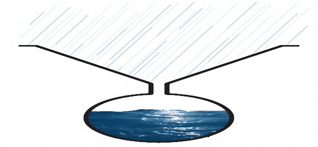
A simple analogy of catchment area to explain Effective Aperture of antenna

We will now proceed to develop the next vital concept (building block) in connection with our endeavor to understand propagation and antennas. Till now we have viewed RX end signals either as Power Flux (W/m²) or Field Strength (V/m). The values we computed are not the absolute amounts of power or voltage as induced into the receiving antenna. They only tell us the flux density prevailing in space near the antenna. The next step for us will be to find a way to compute the actual signal power that is delivered to the RX antenna. This brings us to the concept of Effective Aperture (Ae).

Effective Aperture is akin to a catchment area. The RX Antenna has to work as a fishing net to collect power from the intercepted flux of the incoming radio wave.

If we were to draw another analogy to intuitively follow the concept, let us do it by comparing the EM flux at the RX to rainfall. It can be either be torrential rain (strong signal) or a light drizzle (weak signal). Whatever the case may be, we can measure or quantify rainfall by stating it in millimeters or centimeters of rainfall. But if you want to collect rainwater in a container you would need to know the size of the opening of the container that receives the rain. The larger the size of the opening of the container greater will be the amount of water collected. So the size of the opening is the aperture. With regard to antennas, the concept is identical, but unlike the rainwater collection analogy, it may not be as intuitive.

Without going into mathematical derivations of the Effective Aperture (Ae) of an antenna, let us stick to the core concept. For instance, if we consider a parabolic dish antenna then the above analogy may appear to be similar and quite intuitive. The dish acts as the catchment area and determines the aperture for the overall antenna system. However, for HF, VHF, or UHF antennas which are usually wire antennas or perhaps aggregation of several dipoles as in the case of a Yagi, the catchment area may not be obvious. At this stage, we only need to remember every antenna has an Effective Aperture that might not be shaped like a physical aperture. The reference is the Isotropic antenna.

All other antennas including dipoles, yagis, or whatever also have their own equivalence of apertures called the Effective Apertures. The effective aperture of any antenna can be determined and quantified by multiplying the antenna gain with the Effective Aperture (Ae) of the equivalent Isotropic antenna for the specific frequency (or wavelength). Hence we first need to know the Effective Aperture (Ae) of the Isotropic antenna. Apertures of all other types of antennas can then be calculated if we know their antenna gain.

Now we come to the bottom line. The Effective Aperture (Ae) of an Isotropic antenna is given by the following equation.

Ae = lambda^2/(4pi)

Please remember that the aperture of an antenna is not as tangible and visible as a physical opening or a catchment area as is in the case of our rainwater collection analogy. However, its properties and behavior are quite similar. That is the reason why, in relation to antennas, it is not simply referred to as the aperture but as the Effective Aperture.

We have seen earlier that Power Flux Density at the RX site (Pa) is expressed in W/m². For the sake of clarity, let me recap that Pa is not the RX power picked up by the antenna, it only expresses the power flux density prevailing in free space in the vicinity of the RX antenna. Differentiating these subtle concepts is very important. If we now apply the Effective Aperture (Ae) and its gain (Gr) to the Power Flux Density (Pa), we can compute the amount of power induced into or received by the RX station antenna. Please note that the gain of the receiving antenna (Gr) that we use in our calculations below is not in dB but expressed as gain ratio.

Pr = Pa x Ae x Gr
Pr = (Pt/4πD²) x (λ²/4π) x Gr
Pr = Pt x Gr x λ² / (4πD)²

The above computed received power (Pr) can now be easily converted (by applying the antenna impedance) into either voltage or current that is induced in the receiving antenna and delivered to the transmission line attached to its feed-point.

There is a very important takeaway from the concept of Effective Aperture (Ae). If we examine closely we find that the RX end Power Flux density (Pa) or the E-Field is the same at all radio frequencies. Pa only depends on the distance and the TX power. It remains the same for HF, VHF, UHF, or any other frequency. But the power picked up by (or induced into) the RX antenna is proportionate to the square of the wavelength.

In other words, the shorter the wavelength lesser will be the power induced in the RX antenna and vice-a-versa. Many of us may have heard or read that at UHF or microwave frequencies the signal attenuation due to propagation is higher. This is not entirely true. The signal flux at the RX end in the free space near the vicinity of the receiving antenna is identical irrespective of frequency. It is just that the Effective Aperture (Ae) of the antenna at the RX end becomes smaller with an increase in frequency. Hence the ability of the antenna to pick up induced signal power from the flux gets reduced. To offset the reduction in aperture, VHF and UHF antennas need to be designed for higher gain so as to achieve effective communication.

This is the reason why even a dipole on the HF bands with moderate gain produces a fairly large Effective aperture on account of longer wavelength (λ), whereas, at UHF due to much shorter wavelengths, even a 3-element Yagi may produce a smaller aperture. Hence, to compensate for this, usually, the practically usable UHF Yagi would need to have more elements.

Radio Circuit Path Loss
We also know the relationship between λ and F (λ = c/F). It is now a simple matter to express the Path Loss in dB (Ldb) between the TX and RX stations both using isotropic antennas as follows.

L(dB) = 10Log(Pt/Pr)

If we mathematically combine and rearrange the terms of the above expressions we arrive at the following final equation which a very important formula used extensively to determine various radio circuit path losses. While deriving at the path loss equation, we converted the distance D in meters to Kilometers. We also converted the λ to F, the frequency in Megahertz.

L(dB) = 20logD + 20logF + 32.4

Where

L(dB) = Radio circuit loss in dB (both TX and RX stations using isotropic antennas)
D = Path distance in Km
F = Frequency in MHz.

The above equation gives us expected free space path loss for any distance assuming that Isotropic antennas are used at both ends of the radio circuit. Although it accounts for the antenna aperture relationship with regard to the operating wavelength (λ), it does not account for the gains of antennas on either end of the circuit. To account for antenna gains and derive the effective path loss between two stations using practical antennas, we would need to subtract both antenna gains in dB from the magnitude of free space path loss computed by the above equation. Hence, after accounting for the antenna gains, the equation for free-space path loss will be as under. The transmitter antenna and the receiver antenna gains (in dB) are designated as Gt and Gr respectively.

L(dB) = 20logD + 20logF + 32.4 - Gt - Gr

L(dB) = 20logD + 20logF + 32.4 - Gt - Gr

What we have discussed so far is applicable directly to Free Space propagation and Line of Sight (LOS) propagation conditions. All these concepts are also essential in understanding various other modes of propagation that we will introduce in the following sections.

List of Articles under this Section

Atmospheric impact on VHF Radio Propagation
Atmospheric influence on VHF Radio Propagation The overall influence and impact of atmospheric conditions on VHF radio propagation are quite significant. In this article whenever I mention VHF, it would usually refer to both VHF...
Terrestrial VHF Radio Signal Coverage - LOS
Terrestrial VHF Radio Signal Propagation - LOS Though VHF/UHF radio is very popular, why do the terrestrial VHF radio signal coverage losses grow quickly to curtail the useful range to short distances? This is an important question...
Terrestrial VHF Radio Signal Coverage - BLOS
Terrestrial VHF Radio Signal Propagation - BLOS This is part-2 of the two-part article series on Terrestrial VHF Radio Signal Coverage. This part will focus on Beyond-Line-of-Sight (BLOS) terrestrial VHF radio signal communication,...
VHF Propagation Path Profiler - Web App
Terrestrial VHF Propagation Path Profiler The VHF Propagation Path Profiler presented here is a comprehensive application that allows us to graphically render and mathematically compute various relevant VHF/UHF propagation metrics...