

Solar activity and its influence on Ionosphere
Our sun is a very large celestial body acting as the central pivot of our solar planetary system. It is a continuous source of energy that reaches all planets. The energy released by the sun is multi-faceted and wide-spectrum. This includes electromagnetic radiation across RF, heat, light, X-rays, etc and also sub-atomic particles including electrons, protons, etc that travel at extremely high velocities and contain high kinetic energy. The earth, just like any other planet is heavily influenced by the sun.
The core of the sun is like a gigantic thermo-nuclear reactor producing a core temperature of around 15-16 million °C. The surface of the sun is however much cooler with a temperature of about 5.5-6 thousand °C. Unlike the earth which is a solid body, the sun is a fluid mass comprising of a ball of gasses. The gas (plasma) ball is held together by solar gravity produced due to its mass which prevents the plasma from escaping out. The mass of the solar matter is approximately 100 times greater than the mass of the earth. Consequently, its gravitational force is proportionately greater.
The sun spins on its axis just like the earth. However, due to its fluid plasma composition, the rate of spinning at its equator is different from that at its poles. Unlike the earth (being solid) that rotates as a cohesive body at a fixed angular velocity irrespective of the latitudes, the rotation of the sun is more like the churning of a plasma ball.
The equatorial region of the sun takes about 26.5 days to complete a rotation, whereas, at the higher latitudes away from its equator, the angular rotation becomes progressively slower. The poles of the sun take around 36 days to rotate. This differential rotation of the sun is like the polar ends skidding behind as they try to keep up the pace with the equator.
The Earth and Sun Synergy in Radio Communication
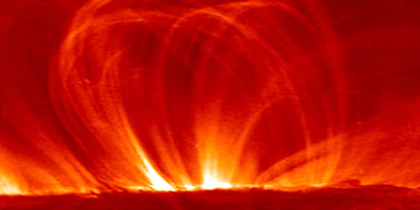
Giant Solar flare loops on sun which are precursors to formation strong solar winds and CME events.
A full cycle of geometric reorientation of the solar magnetic field takes around 22 years. Every half cycle of this phenomenon results in a reversal of magnetic field polarity. Therefore, the 11 year period corresponding to each half-cycle becomes a matter of special interest to us. Though it is a half cycle on the sun, we on earth, call it the 11-year solar cycle because we experience an 11-year cyclic phenomenon that significantly determines the properties and behavior of the ionosphere on earth.
Some of the other important routine physical phenomena of the sun that are of special interest to us are the regular but unpredictable eruption of a large quantum of energy and particle matter from its outer surface. These are observed on earth through telescopes and appear as erupting spots like the bursting of pimples. However, these erupting spots (or pimples) are huge in size. Some of them are 75000-1000000 kilometers in diameter. They are called the Sunspots. Astronomers have been counting the occurrence of sunspots for almost 250 years. Ever since the advent of radio communication, scientists have discovered a close correlation between the appearance of these sunspots to the viability of reliable HF radio communication on earth.
Although the sun spews out a lot of matter and energy continuously providing a steady-state solar emission condition that determines a base state ionization of our ionosphere, the additional emission of energy and particle matter from the erupting sunspots directly influence the properties of the ionosphere by creating several types of random as well as cyclic variations of HF radio propagation conditions.
As we build up up narrative in this article, we will examine various day-to-day phenomena occurring on the sun as well as the longer-term effects of the solar magnetic cycle. We will correlate their influence on various factors that influence HF radio propagation on earth. Read on…
The Sunspot Number – SSN
The Sunspots have been of great interest to those involved with HF radio communication. The counting of sunspot occurrences is aggregated on a daily basis to arrive a what is known as the Sunspot Number. We have a well-established protocol for counting sunspots and the method that is followed is called Wolf’s sunspot count. This is based on the work done by the scientists way back in the 1840s who suggested a viable algorithm. without going into the details of Wolf’s method, for our purpose, it would suffice to daily sunspot counts are made by several observatories around the world.
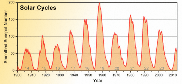
Variation of SSN in accordance with 11-year Solar cycle that defines HF radio communication prospects on earth.
However, the problem is that the ionospheric behavior leading to HF propagation does not respond to this zig-zap variation of sunspot numbers. To lend further clarity and sanity to the sunspot pattern data, the sunspot number plot is further smoothed out using a mathematical method called the Lincoln-McNish smoothing algorithm. This results in what we call the Smoothed Sunspot Number (SSN).
SSN provides us a far better correlation between the sunspots and ionospheric behavior. SSN is often used reasonably well for making a long-term average forecast of the probability of HF radio propagation conditions. However, only depending on SSN for propagation forecasting has several shortcomings. The process can be further refined using modern methods and available data to make far better forecasts that are more accurate even on a short-term and daily basis. However, to achieve this we need to look beyond just the SSN.
Before we discuss further, we need to quickly appreciate a few important factors that render pure SSN based forecasts to be not so effective. We will describe the ionosphere in greater detail later in this article but is important to know that the earth’s ionosphere is huge and it has a very huge inertia that resists change. Therefore a quick change in SSN will make little or no change to the ionosphere or the associated HF propagation conditions.
Moreover, when a sunspot eruption occurs, it not only produces electromagnetic energy but also spews a huge volume of sub-atomic particle matter. The quantum, as well as the ratio of the energy to the matter components of a sunspot eruption, may vary greatly. Some eruptions may produce more energy and fewer particles while others may do the opposite. Hence, it will be a fallacy to treat every sunspot as identical.
Another important factor is that other than the regular sunspots, the sun may occasionally produce gigantic eruptions that eject the colossal amount of particle matter along with energy. These events are called Coronal Mass ejection (CME). When a CME occurs, the ejected matter is thrown out with a force that is several orders of magnitude greater than what happens with regular sunspots. This results in a very high kinetic energy particle that travels out at extremely high velocities. Hence the particle matter from a CME will reach the earth quicker than the particles from a sunspot eruption. In other words, the effect of a CME on the earth’s ionosphere may occur much earlier than expected.
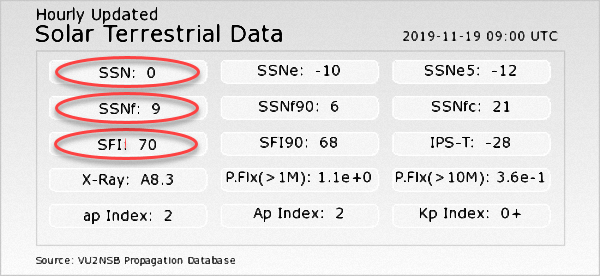
Typical set of Solar data metrics measured or derived from radiation measurements.
Light, heat, and X-ray are some of the primary energy compositions produced by the sun. The light and heat do not noticeably influence the ionosphere, whereas, X-ray emission is a major factor responsible for ionization. On the other hand, the high energy (higher velocity) proton flux ejection from the sun is another vital factor influencing ionospheric behavior.
All the above factors add to the complexity. The X-ray energy travels at the speed of light and hence covers the distance between the sun and the earth (150 million kilometers) in approximately 500 seconds (about 8.5 minutes). The effects due to X-ray start altering the ionosphere after 8.5 minutes. However, the proton flux from either the sunspots or CME, both traveling at markedly different velocities could take from 2-8 days to reach the earth. The high-velocity CME particles may reach earth in 2-3 days and start affecting us after that. The Sunspot particle matter ejections traveling relatively slower typically reach the earth in 5-8 days. The particle flow through the inter-planetary space that engulfs the earth is like wind and hence we call it the solar wind, whereas, the super-high velocity particle from a CME results in what we call the solar storm.
The Solar flux Index – SFI
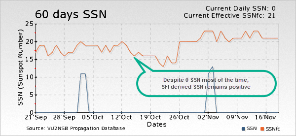
The counted SSN vs the SFI derived SSN which provides a better indicator of Ionospheric activity.
Being a real-time parameter being measured at close proximity to the earth, the SFI values show a quick correlation to the changes in the ionosphere. Although SFI does not account directly account for the effects of particle matter ejected from the sun but it is a fairly accurate approximation that leads to the ability of forecasting ionospheric behavior from a general HF radio communication perspective. Moreover, SFI and the SSN follow a general trend of variation that is quite similar. By using mathematical correlation, the Equivalent SSN can be calculated from the measured SFI.
Working with SFI rather than the counted SSN gives us a far more accurate correlation to the ionospheric behavior. In other words, the SFI derived SSN as against the counted SSN allows us to follow and forecast ionospheric behavior far better. This type of SFI derived SSN is often referred to as SSN(10.7) or SSN(f). Rather than working with SFI directly, the derived value SSN(10.7) provides us with greater flexibility by allowing us to apply SSN(10.7) to all existing propagation forecasting models and also achieve better and more reliable forecasts.
Solar Activity – The way it affects us
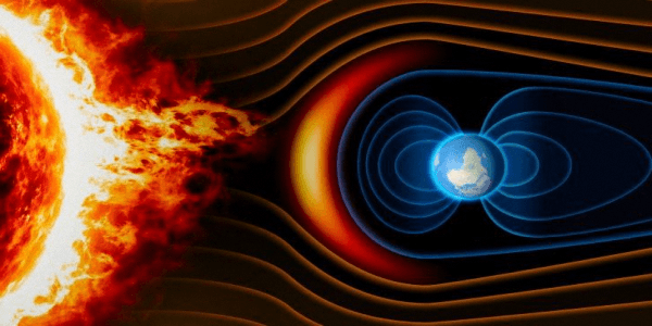
A graphical depiction of Solar winds as they flow around Earth and the Magnetosphere.
For now, let us briefly introduce ourselves to some of these phenomena and their effects. The two broad components of solar emissions (notwithstanding several other subtle factors) are the EM wave energy emissions and the sub-atomic particle emissions. Let us see how they produce different kinds of effects to influence our ionosphere and the overall HF propagation scenario in general.
The EM emissions, of which we are primarily concerned with the X-Ray component, are produced by the sun continuously at more or less a steady-state level along with additional spurts of X-Ray intensity caused on account of sunspots and CME. This radiated energy traveling at the velocity of light reaches the earth in about 8.5 minutes. As they penetrate the highly rarified upper layer of our atmosphere and impinge on the rarified gases, they produce ionization due to the physical phenomena of photo-ionization. This creates negative and positive ions consisting of free electrons and protons by knocking out electrons from the atoms.
The net result is that the upper atmosphere gasses get ionized and start acting like a plasma cloud. The density of the plasma is proportionate to the intensity of the X-Ray from the sun. As long as the X-Ray emissions continue, the ionization is maintained. These ionized gases of the plasma tend to form multiple layers of concentrated ionization in the upper atmosphere. These sets of ionized layers are collectively called the Ionosphere.
On the other hand, the ejected particle mass that travels at velocities is typically in the range of 200-400 Km/sec or even more in the event of large CME. Extremely high particle velocity under CME conditions gives rise to what we call the Solar Storm. These particles, when ejected from the sun, form a huge mass and a large collective volume. Since they travel at such high velocities, even though they are of sub-atomic mass, they acquire very high kinetic energies. Basic school level physics tells us that kinetic energy is…
Ke = 1/2 x m x V2
As the solar wind or storm travels towards the earth and encounters the earth’s magnetic field (the magnetosphere), their path of travel tends to get diverted till the direction of travel of most particles align themselves tangential (parallel) to the magnetic field lines. This region where the transition of direction happens in the magnetosphere is called the Bow-shock region. A small percentage of these particles, however, penetrate deep through the magnetosphere to reach our upper atmosphere. They usually penetrate deeper till they start colliding with the molecules and atoms of atmospheric gasses, whereby they too contribute to ionization thus strengthening the plasma density of some layers of the ionosphere.

Typical creation of Aurora at the poles due to solar storms.
In the process, they produce two major phenomena that affect our HF propagation behavior. Firstly, their interaction with the magnetic field lines in the upper region of our magnetosphere, causes the magnetic field lines to be disturbed. This, in turn, results in creating turbulence, unevenness, and other anomalies in the usually placid layers of our ionosphere. As the result, the propagating radio waves that refract from the ionosphere to achieve skip mode communication become a little unpredictable and haphazard causing excessive signal fading and path losses thus reducing HF communication reliability across the board.
The second important effect of a large burst of a solar emitted particle is to produce an excessive concentration of ionized particles that now travel to the north and the south poles. Since the earth’s magnetic lines converge at the poles, these particles gradually reach lower altitudes as they approach the poles. Somewhere near the poles, they travel along the magnetic lines low enough to encounter a denser atmosphere. Due to the higher density of gasses at lower heights, they start colliding frequently with the gas molecules. This produces photo-ionization and produces light emissions from the atmospheric gasses.
Since all this happens near the poles, the net effect is to produce an atmospheric glow called the Aurora. Though the Aurora is visually spectacular, they comprise of ionized gasses. As a result of this enhanced ionization, the Auroral region at both the north and south poles begin to affect radio communication. HF communication via trans-polar great-circle paths suffers due to additional propagation losses.
Even when propagation might be possible, a strong Aurora will produce increased fading and signal distortion. On the upper HF, VHF, and UHF bands, the Auroral columns quite often act as large reflectors (as if like very turbulent vertical ionosphere sections). They often reflect radio waves to provide propagation into regions that might not be normally possible on those bands. However, the downside is that Auroral refractions undergo excessive phase shifts and selective frequency fading to render the radio signal highly distorted.
Getting to know the Ionosphere
After having had a look at the Free Space and Ground Wave propagation models in our previous articles, we are now set to step into the realms of SkyWave propagation which is the most vital mode of propagation that renders absolutely unique and amazing capabilities to HF bands. But before we step into the world of Sky Waves, let us lay the foundations by understanding the basics of the Ionosphere which is formed in the upper part of the earth’s atmosphere. Let us now review the atmosphere and the ionosphere.
Very often we tend to believe that the atmosphere is just the region of air above us that harbors the wind, rain, snow, and other effects of our weather system. That is not entirely true. What we so often intuitively call the atmosphere is actually a rather small portion of the atmosphere and is technically called the Troposphere. Our atmosphere extends is huge and extends several hundreds of kilometers above the earth and is segregated into several discrete regions based on their unique properties. We will gradually lift the mist as we continue our narrative.
While radio waves traveling in free space have little or no extraneous influence to affect them, the radio waves traveling in the earth’s atmosphere may be influenced by many physical phenomena that might alter or affect their properties and behavior. At one time or another, all of us might have experienced various problems with radio waves communication, even while listening to broadcast radio, caused by various atmospheric conditions. However, in this article, we will restrict our focus primarily to the Ionospheric layers of the atmosphere because of their predominant influence on HF radio communication.
Before we start digging deeper into the properties and behavior of the Ionosphere, let us take a sneak preview of the earth’s atmosphere in general. This will enable us to understand the Ionosphere a little better.
The anatomy of the Atmosphere
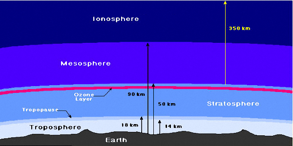
Classification of Atmospheric regions above earth.
The lower portion of the atmosphere where the typical rate of temperature reduction with height is fairly uniform is called the Troposphere. The Troposphere extends from the surface of the earth up to a height of 10-14km or so. This is the part of the atmosphere that contains the right mixture of gases to support life and is also responsible for our planetary weather. The point just above the Troposphere at which the temperature stabilizes is called the Tropopause and is to be found at around 12-18km above the earth’s surface.
Upwards of Tropopause to a height of about 40-50km, we have the Stratosphere. This is the part of the atmosphere where aircraft fly as the air is thinner and hence there is less friction and drag, allowing the aircraft to fly faster and use less fuel. Temperature is fairly constant but does tend to actually increase as the top of the stratosphere is reached (the Stratopause). The next higher layers form the Mesosphere and the Thermosphere region, which extends up to 650km or beyond). It is the set of several Ionospheric layers that reside partially within the Mesosphere and largely within the Thermosphere happens to be the HF radio operator’s greatest asset.
Troposphere
Almost all weather phenomena take place in the Troposphere. The temperature in this region decreases rapidly with altitude. Clouds form, and there may be a lot of turbulence because of variations in temperature, pressure, and density. Although these conditions affect the propagation of radio waves at VHF/UHF and microwave frequencies, they do not have any noticeable effect on HF radio propagation. There is a thin atmospheric buffer zone above the Troposphere which is called the Tropopause. Since Troposphere plays no role in HF communication, we will leave it alone and move on.Stratosphere
The Stratosphere is located between the Troposphere (above the Tropopause) and the Mesosphere/Thermosphere. The temperature throughout the Tropospheric region is almost constant and there is little water vapor present. The airflow is non-turbulent, horizontal, and laminar. At the upper portion of the Stratosphere lies the Ozone layer which is responsible for absorbing the UV radiations from the sun. The Stratosphere has almost no effect on radio wave propagation. The stratosphere is primarily a region that due to its placid behavior is well suited for airliners to fly.Mesosphere
This is the layer of the earth’s atmosphere that lies just above the Stratosphere. The temperatures in the Mesosphere decrease with increasing height. The upper boundary of the mesosphere is called the Mesopause, which can be the coldest naturally occurring place in the earth’s atmosphere with temperatures below -140 °C. The mesosphere is a region that hosts the Ionospheric D-layer as we will see later.Thermosphere
The Thermosphere is the upper atmospheric region above the Mesosphere. This is the region that extends to 600 km in height. The temperature rises (as high as 2000 °C at the top) with an increase in altitude which is also dependent on solar activity. The concentration of gas molecules in this region is very low in this rarified portion of the upper atmosphere. We, as HF radio operators are really interested in this region because it hosts the most important Ionospheric layers, the E-layer and the F-layers (F1 and F2) which are the principal facilitators of HF radio communication.Ionosphere
The Ionosphere is not an independent atmospheric region. Unlike all the atmospheric regions that are integral to the earth’s atmospheric system, the Ionosphere does not exist by itself. The Ionospheric layers that we are interested in are actually created within and are hosted by the Mesosphere and the Thermosphere. Both the Mesosphere and the Thermosphere consist of stratified layers of various different gases like Nitric-oxide, Nitrogen, Oxygen, Hydrogen, Helium, and several other rare molecules like Neon, Xenon, Argon, Krypton, etc. Solar radiations like UV, X-ray, and several types of cosmic particles are responsible for the ionization of gas molecules in these upper atmospheric regions. The free electrons produced due to the ionization of gases interact with the magnetic field of the earth to produce a concentration of charged ions at certain altitudes within the Mesosphere and the Thermosphere resulting in what we call the Ionosphere. Without the presence of solar and other galactic radiations, ionization would not be sustainable. In other words, the Ionosphere cannot exist without continuous solar radiation.The anatomy of the Ionosphere
The Ionosphere is comprised of several layers of ionized gases located from 60 to 350km (approx) above the earth’s surface and are hosted by the Mesosphere and the Thermosphere. These layers can combine, split or change their characteristics depending on the intensity of solar radiation and are also influenced by other solar activities.
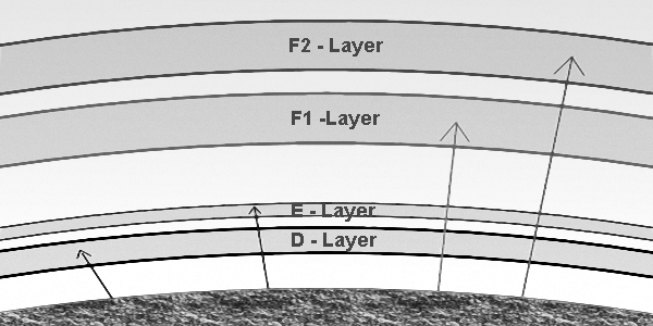
Typical layers formed in the Ionosphere.
Under normal circumstances, radiations from the sun consisting of intense UV and X-ray (apart from light and heat) illuminates the daylight side of the earth and enter the upper atmosphere to travel downwards towards the earth. In their path, these radiations encounter various gases in the Thermosphere and the Mesosphere. Both UV and X-ray flux contain high energy. When these UV or X-ray photons come in contact with the gases in the Thermosphere they transfer some of their energy to the gas molecules and manage to knock off an electron in the process. Light and heat (Infra-red) flux do not have enough photon energy to cause ionization. This phenomenon is called Photo Ionization.
The continuous process of photo-ionization results in the creation of high levels of ionization and electron charge density. Some of the free electrons do collide again with electron-deficient atoms to recombine into a non-ionized state. The rate of ionization and the rate of recombination equalize at a level thus producing a steady state of ionized layer charge density. Of course, the charge density will vary with the solar radiation intensity. The higher the intensity of solar radiation higher is the ionization density.
Let us now take a quick look at the various layers of the Ionosphere at varying heights above the ground. We will take a glimpse of the basic principles of the formation of steady-state ionospheric layers. More intricate ionospheric phenomena resulting in the account of Solar flares, Coronal Mass ejection (CME), solar storms, Solar cycles, declination of the earth, seasons, and diurnal variations will be examined later in separate articles.
D-Layer
The lowest level is the D-layer (60 to 90 km), which does not contribute to HF propagation, but actually works against it by absorbing most of the energy in the transmitted wave. The normal height of the D-layer is approximately 90 km but can extend down to 60 km during periods of high solar activity. At night, in the absence of solar radiation, the electron density of the D-layer drops down by a factor of 10 or more. Since it does not adversely affect nighttime propagation, it is often considered to be non-existent.However, in reality, the D-layer does not completely disappear at night. It maintains very low electron density which is sustained by radiation from other nighttime galactic sources. The dominant gases in the D-layer are Nitric Oxide and Hydrogen, which are forced to emit ultra-violet and infrared emissions during the daytime hours. Ionization is mainly by hard X-rays. These gases cannot hold ionization very long; hence, the D layer practically disappears rapidly after local sunset only to reappear after dawn.
E-Layer
The E-layer (90 to 120 km) ha a nominal height of 110 km, the region where the ionization charge density is at its maximum. E-layer is present during the day and almost disappears at night in a manner similar to the D-layer. However, during the day it contributes to mold the propagation behavior of radio waves at mid-HF frequencies. At higher HF frequencies the radio wave generally penetrates the E-layer comfortably with minimal losses and travels to reach the F-layer which plays the role in providing Ionospheric skip. It can sometimes produce sporadic HF propagation due to soft X-ray emission and ultra-violet stimulation of Molecular oxygen (O2). At night time, the Sporadic-E (Es) occurs due to electrons and meteor bombardment. Sporadic-E propagation is still not well understood and still is being investigated by planetary scientists.F-Layer (F1 and F2)
The F1 and F2 layers (150 to 350 km) are the layers that mostly contribute to HF propagation. The nominal height of the F1 layer is about 200 km while that of F2 is 300 km. These heights vary with solar activity. At night due to the absence of the ionizing radiations from the sun, the F1 layer charge density reduces an extent where it merges with the F2 layer to form a common F-layer.At night the combined F-layer continues to exist and maintain a significant charge density. This is because of the extreme rarified atmospheric gas density at the high altitude of the Thermosphere. Due to the rarified atmosphere, the electrons and the positive ions do not easily collide to recombine. The recombination time is quite large. Hence, by the time sufficient charge recombination takes place, the night is over and it is daylight once again.
Although the F-layer night time ionization density progressively reduces with the passage of night, it is still sufficient to maintain viable F-layer skip mode HF communication. The interesting effect is that at day time, the higher frequencies are suitable for F-layer skip while at night lower frequencies start working better and the higher frequency bands become inoperable. This leads us to the concept of Maximum Usable Frequency (MUF) which we will discuss later in dedicated articles. Dominant gases are Hydrogen and Helium, with trace components of Neon, Argon, Xenon, and Krypton. Ionization is mostly via solar UV and X-Ray emissions.


(25 votes, Rating: 5.00) - Please vote the article with your valuable star rating. Thanks! Basu (VU2NSB)


Ham Rig Reviews Coming Soon
SSN SSNf(10.7) – Real-time Solar Data


