Terrestrial VHF Propagation Path Profiler
For graphical signal path rendering and numerical computations over the terrain profile, not only the terrain topology but also the terrain bulge due to the curvature of the earth is factored into the computations. Various input variables like the antenna height over ground, their gain, etc can be set. The frequency band and the TX power levels are also settable. This signal path rendition is not an over-simplified straight line that some people often assume but it accounts for the Fresnel zone envelope thus rendering a curved path over obstacles when workable SNR can be produced at the receiving end.
Another niche feature of the VHF propagation path profiler application is that the atmospheric refractivity gradient (ΔN/ΔH) that leads to various magnitudes of super-refraction can also be set. The resulting computations and the graphical profile display rendering include these effects.
The VHF Propagation Path Profiler presented below may be used to determine VHF/UHF propagation prospects between any two locations under the influence of a variety of variables thus rendering a fairly accurate assessment. The propagation path loss in dB including various sub-components of its net value, the RX end signal strength in dBm, the expected RX S-units, and the RX side signal-to-noise ratio (SNR) are computed for the analyzed communication path.
Before you begin, please scroll down below the application block presented here and carefully read and understand the operating instructions. A step-by-step procedure of how to use the VHF Propagation Path Profiler has been provided along with several graphics to make it easy for you to familiarize yourself with the application… All operating steps have been explained in simple terms…
Application Operating Instructions (Please read…)
There are essentially three parts to the VHF Propagation Path Profiler application usage. They are listed below and thereafter each part of the operation is further explained…
- Part 1 – Map setting of TX and RX locations.
- Part 2 – Default profile rendering and computation.
- Part 3 – Applying communication variables and re-rendering.
Part 1 – Map setting of TX and RX locations
Before the VHF propagation path Profiler application could do calculations, the TX (transmitter) and the RX (receiver) points have to be specified. Generally, the TX point is your own location while the RX point is the other DX location. Both these points have to be specified on the map section of the application provided above.
Step 1 – Set map to Home location
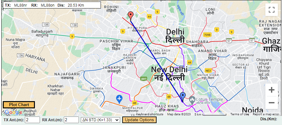
When the application initially loads, it displays a fully zoomed-out world map. One could use the map controls to zoom and pan to your desired starting point. However, in most cases, we might be interested in our own home locations irrespective of where we might be located in the world. Under normal circumstances, VHF/UHF terrestrial communication is restricted to several tens of kilometers usually, or at best may extend to several hundred Kilometers (perhaps 1K-2K Km) under unusual atmospheric refraction conditions… Therefore, it would be far more convenient if the map could zoom and pan by itself to your home location… We have provided you with exactly this feature… Check the image below. At the top left corner, there is a button marked Set Map to Home QTH. Click the button and your map will zoom and pan to your location.The map sets to your Home QTH… Now, you may proceed to the second step given below… However, should you wish to go back to the full world map at this stage, you may Double-Click mouse anywhere on the map canvas and accept the confirmation dialog to reset the application to its default state. The original map status before this Step-1 will be restored.

The illustration depicts the VHF Propagation Path Profiler state at the beginning. This is the default opening window.
Step 2 - Set the TX location on the map
Once your map has been set to your home region, you may decide where to set your TX station point. If needed, you may do some finer panning or zooming to find your desired TX location. Don't be too finicky about choosing the exact street, block, or house. It doesn't matter even if your selected TX point is a few blocks away... Now, hopefully, you have found the desired location. Proceed to do the following...- Most Important - Do NOT at any stage Double-Click on the map canvas unless you want to start all over again. This action will master reset the application. It will remove any TX or RX point settings that you might have made and reset the map canvas to the default zoomed-out world map... Of course, the application will throw up a confirmation warning to prevent any inadvertent reset.
- After you decide your TX location, move the mouse pointer to that location and Left-Click. A red marker will be placed at that location designating your TX location. A narrow window appears near the top-left corner of the map. It will display the TX location Maidenhead Gridsquare. If you hover the mouse pointer over the TX marker, it will display the exact latitude and longitude. On touchscreen devices, instead of mouse hover you will need to single-tap on the marker to display the lat/long information.
- Should you wish you make fine adjustments to the TX location, you may hold down the mouse pointer on the marker and slowly drag it around according to your choice. The latitude and longitude display will continually update as you drag the marker.
- At this stage, should you for any reason wish to remove the TX marker and place it elsewhere, then simply Double-Click mouse on top of the TX marker. Remember NOT to Double-Click on the map canvas area.
- While setting your TX marker that you placed, if you inadvertently Left-Click on the map again then another marker in blue color will appear along with a line joining the 2 markers. This new marker will designate your RX location. However, since you were not intending to place this second RX marker at this stage, you could remove the blue RX marker and the line by double-clicking on top of the unwanted marker.
- Finally, once you are satisfied that the red marker designating your TX site is properly placed, you may proceed to Step-3 below.
TX and RX site markers along with their geodesic path have been setup as depicted in this illustration.
Step 3 - Set the RX location on the map
The procedure for placing the RX location marker is identical to the TX marker setup procedure described above. Hence, we will not elaborate on the procedure again. However, there are a few things that you need to know...- Choose the desired RX location on the map and Left-Click mouse to place the blue colored RX marker.
- When the blue RX marker appears, a geodesic path line in blue color also appears that connects the red TX marker and blue RX marker locations.
- As in the case of the TX marker, the new blue RX marker can also be dragged and moved around on the canvas. Its latitude and longitude are also visible on mouse hover, or by doing a single tap on the marker in the case of touchscreen devices. The left-top end window on the map now also displays the Maidenhead Gridsquare of the RX marker along with the total path distance. This information is dynamically updated if you drag the RX marker.
- As in the case of the TX marker, the RX marker may if desired be removed by Double-Click on top of the marker. However, please note that after the RX marker has been placed the earlier placed TX marker is no more draggable or deletable. Should you for any reason wish to edit or delete the red TX marker, you will first have to remove the RX marker before the TX marker becomes editable once again.
- Once you are satisfied with both marker placements, this part of the procedure may be considered to be complete. You may proceed to the next part of the procedure given below.
Part 2 - Default profile rendering and computation
After having completed the Part-1 of the map setting procedure, we will now perform the default profile rendering procedure as explained below...
- At this stage, you will find that a new button marked as Plot Chart would have appeared near the lower-left end of the map canvas.
- Click on the Plot Chart button now... voila! ... The Elevation Profile chart area at the lower end of the application now displays a full rendering of the VHF Propagation Path Profile. The left end of the elevation path profile indicates the TX side, while the right end is the RX side. A new window pops up on the left side of the map canvas showing the propagation metrics summary.
- After you click the Plot Chart button and computations are performed, the blue-colored RX marker turns green indicating that the path is now active. You will no more be able to edit the markers on the map. The path layout may be deemed to b frozen. Of course, you may pan or zoom the map canvas as you wish. At any time should you wish to start all over again by setting a new communication path circuit, you may do so by a Double-Click on the map canvas. This will reset the application and set all parameters to default.
- The entire thing may appear to be daunting at first sight but don't worry. We will walk you through all aspects of the chart as well as the propagation summary.
- You may roll the mouse pointer across the VHF Propagation Profile chart and notice that just above the chart, at the top-right side the distance from the TX side, the Elevation of the terrain above mean sea level (AMSL), and the signal envelope path height above mean sea level (AMSL) will be dynamically displayed. The elevation profile displays the true graphical rendering of the topological terrain profile across the signal communication path that is indicated by the blue geodesic path line on the map.
- You might also notice that there is a red color X at the top-right corner of the propagation summary window on the map. This can be clicked to close the summary window. When this window closes, a button marked Click for Propagation Data appears at the bottom-center of the Elevation Profile chart. Click this button to re-open the window. Normally, on laptops and desktops, it may not be needed, however, on smaller devices this window may cover most of the map area. To access the underlying map layer you may want to close the summary window temporarily.
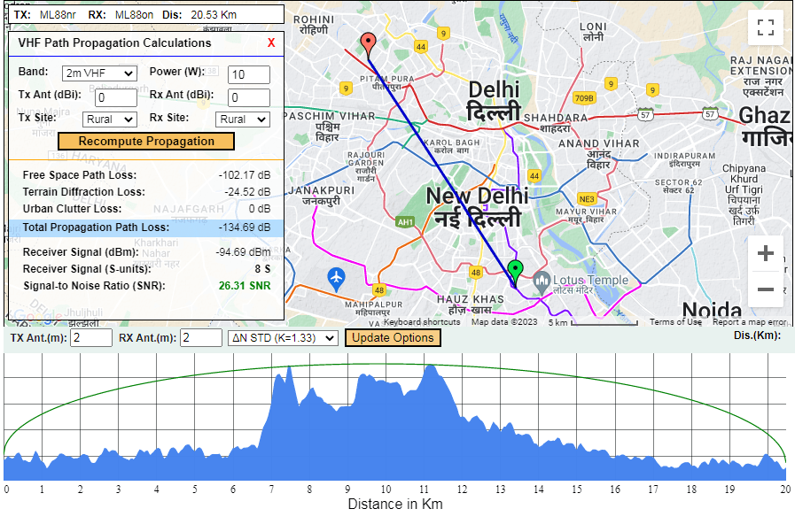
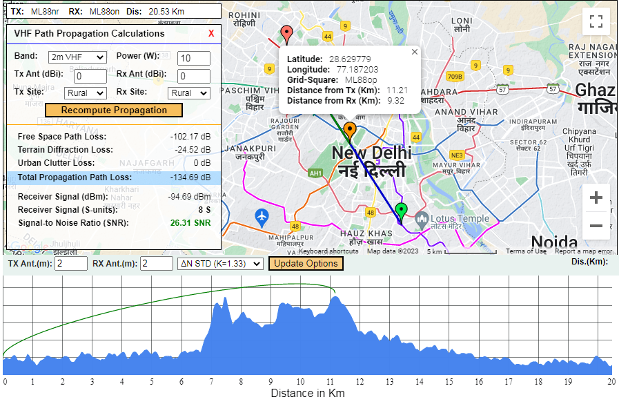
This illustration depicts a typical default phase computation of VHF propagation path profile computations and graphical rendering along with elevation map of the terrain features along the path.
So far so good but are we done? ... No! not as yet... What we have got so far is the elevation profile and the propagation summary rendered using default parameters. In all probability, the default setting may not conform to your real operating conditions. For instance, your antenna height or gain may be different, the TX power level may also differ, the nature of your TX and RX sites may be entirely different, and so on... We must account for these factors. However, before we do it let us first see what are our default conditions. Check out the default conditions listed below...
- Operating Band (λ):- 2m (144MHz band).
- Antenna Height above ground (AGL):- TX antenna: 2m and RX antenna: 2m.
- Antenna Gain in dBi:- TX antenna: 0 dBi and RX antenna: 0 dBi.
- Transmitter Power Level (W):- 10 Watts.
- TX and RX Site Profile:- TX site: Rural and RX site: Rural.
- Atmospheric Vertical Refractivity Gradient (ΔN/ΔH) based Earth Radius Factor (K):- Standard gradient K: 1.33 (More explanation later)
The above-cited set of default parameters is likely to be quite different from your actual conditions. Hence, to compute an accurate analysis based on your true conditions we would now need to update these parameters and Recompute Propagation. We will do it in the following Part-3 of the procedure.
Part 3 - Applying communication variables and re-rendering
This is quite a straightforward procedure. We already have the default rendering available. Now, you need to make proper selections of settable parameters in the VHF Path Propagation Summary window. You also need to set TX and RX antenna heights in the Options Bar available below the map and above the elevation profile chart on the left side.
All these parametric settings can be done either using dropdown selectors or through number fields using Up/Down selector buttons... At this stage, for many of us who do not understand much about atmospheric gradients and super-refraction conditions, I suggest that you leave the Atmosphere Setting to the default ΔN STD K=1.33 for the time being. This setting represents the standard atmospheric conditions that prevail most of the time at any location around the world.
However, to leverage the VHF Propagation Path Profiler application capability at a later stage I would suggest that you read the article Atmospheric impact on VHF Radio Propagation. It might be a time well spent because you will then be able to understand Super-Refraction conditions. Thereafter, you will be equipped to find and compute VHF/UHF terrestrial DX prospects under different atmospheric refractivity gradient conditions. Wouldn't it be great to be able to find VHF DX propagation prospects over several hundred or even thousands of Km distances? Something that many of us thought was perhaps not possible...
Although this application can reasonably accurately find VHF propagation path prospects under different atmospheric refraction conditions resulting in the bending of VHF/UHF radio waves, it does not cover the phenomenon of atmospheric ducts of any kind. Usually, a duct formation whether it is a surface duct, an elevated duct, or an evaporation duct over large water bodies like the sea may lead to short/medium duration strong DX VHF/UHF propagation prospects.
Here are a few important notes to assist in setting up various parameters before Recomputing...
- Band Setting: This is self-explanatory. Choose either 2m, 70cm, 23cm, or 13cm.
- Power Setting: Set to applicable value between 1W and 200W.
- Antenna Heights: Set independently each of the TX and RX antenna heights above ground level (AGL) between 2m and 200m.
- Antenna Gains: Set independently each of the TX and RX antenna gains between -20dBi to +30dBi. Now, one might wonder why we have a choice to select negative antenna gains. That is because although many of us might be blissfully unaware, there are plenty of commonly used VHF/UHF antennas that provide negative gain. Especially, if you are carrying an HT then your rig is bound to have negative antenna gain... Check out some of the facts below and apply them to your antenna gain selection if relevant...
- Short Stubby Rubber Duck Antenna: -20 to -15 dBi.
- Normal Length Rubber Duck Antenna: -15 to -10 dBi.
- Whip Antenna mounted on HT without GP: -8 to -3 dBi.
- Outdoor 1/4 λ GP Antenna including cable loss: -3 to +1 dBi.
- And So on...
- Short Stubby Rubber Duck Antenna: -20 to -15 dBi.
- TX/RX Site Settings: Set independent Site options for TX and RX locations based on Rural, Urban, or Metro locations. Choose Rural if the site is in a rural or a vast open area of a few square kilometers. Choose Urban in the case of either sub-urban or small and medium-sized cities with regular 2-3 story buildings. Choose Metro if the site falls in a large or metropolitan city with tall and high-rise buildings.
- Please Note: While choosing TX or RX site type, choose between Rural, Urban, or Metro based on the site surroundings. If the height of the building cluster within a couple of hundred meters around the TX/RX site in the direction of the signal path meets the site type criteria then select that type. For instance, even in a metropolitan city if the TX/RX site lies in a relatively wide open area with no tall buildings (< 10-12m high) then select Urban instead of Metro for that site location.
- Important: Please remember that the building clutter losses applied to the TX/RX site type selections of either Urban or Metro are approximations. The VHF Propagation Path Profiler application has no means of knowing the exact density of building clutter, the real heights of structures, or the exact proximity of the sites to the nearest obstructing building. Therefore the computed signal metrics due to structural clutter diffraction may be off the mark by up to ±5-10 dB of SNR due to these factors. A reasonable SNR margin must be kept in mind to account for this ambiguity.
- Atmospheric Refractive Condition: Settable in several steps from STD (K=1.33), MED (K=3), HI (K=9), SUP (K=18), V.SUP (K=35), or MAGIC (K>99)... There is also a Flat Earth selection option for general visualization of terrain profile devoid of the terrestrial bulge of the spherical earth... If not familiar with this concept, leave it at the default STD setting.
After you have made all the required settings as explained above, hit the Recompute Propagation button in the Propagation Summary window. A newly updated elevation profile chart will be generated along with updated signal information in the propagation summary window.
How to interpret and setup propagation computations
To interpret propagation computations and resulting prospects, you may check both the elevation profile chart as well as communication circuit link budget metrics updated in the Propagation Summary window.
The VHF propagation path elevation profile chart provides a graphical overview of the terrain topology between the TX and RX sites. The terrain profile visualization includes the curvature of the terrain due to the Earth's spherical bulge. The communication link path is displayed either as a red or green colored arc. The shape of the path includes a partial ellipsoidal curvature in accordance with the shape of the manifesting Fresnel Zone envelope. On account of their heights, the terrain features between TX and RX sites could result in direct LOS path obstruction. Therefore the signal path has to diffract over the terrain feature obstruction. The diffraction results in additional path losses in comparison to free-space losses. However, if the aggregate of obstructive diffraction losses over the terrain features may still be within tolerable limits to allow the communication link to function... The graphical rendition of such signal paths appears as elliptically curved and tends to go over the terrain feature obstruction.
With the given TX power level, wavelength, antenna gain, etc if the RX side SNR is good enough for communication then the curved communication path is displayed in Green. On the other hand, if the aggregate terrain diffraction losses are more than acceptable to produce a poor SNR at RX then the path is displayed in Red color and so is the SNR value in the summary window. Since the compound diffraction losses could be excessive, the curvature of the corresponding path profile may not be enough to go over the highest terrain peak. Therefore, such red-colored, unusable paths will tend to cut through the terrain features instead of clearing and going over them.
Now, let us take a look at the communication link budget calculated and presented in the propagation summary window...
Here is a practical example presented where we find that there is a communication link budget shortfall due to the obstructive terrain profile, and urban clutter, as well as the limitations of TX and RX station setups... Let's take a closer look...
You may find it interesting that the unworkable scenario presented in the illustration below is for the same path and TX/RX locations that we see in the previous illustration showing default results. In the previous default scenario, the propagation was possible with a good SNR margin even though both TX and RX antennas were only at 2m heights AGL and their gains were 0dBi. In the scenario below, we increased TX and RX antenna heights to 25m and 20m respectively. We set the TX antenna gain to +3dBi and set the TX power to 25W instead of 10W default... Yet the communication link is unworkable. What gives? ... The answer is that since both TX and RX sites lie in the metropolitan area of New Delhi, we designated both TX and RX sites as Metro instead of the default Rural condition. Additional diffraction losses due to building clutter caused the communication link to fail.
Does this application help us to find a solution by overcoming various limitations? ... I would say it does! We will examine parameters and try to establish suitable communication parameters between the two given locations... Read on...
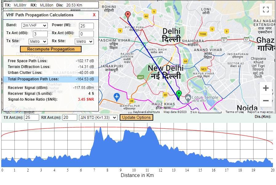
The illustration shows the condition in which the point-to-point propagation prospects do not exist even with TX and RX antennas raised well above ground. The SNR shortfall occurs due to Metro site environments at both TX and RX locations.
It is evident from the elevation profile chart displayed above that the communication link is not practical. Despite the reasonably high antennas on both sides, the high aggregate fresnel zone obstruction losses are perhaps the major contributory factor causing link failure. The signal path is in red and it falls just short of clearing the terrain obstruction... If you look are the computed signal strength and the ensuing SNR values, you will discover that the link budget shortfall is very marginal... Can the link be tweaked to establish communication? Perhaps yes! ... Let's explore...
We have several options to make the communication link workable. We may either increase the TX power level from 25W to at least 75-80W or increase antenna gain and/or heights on either/both the TX and RX sites. The combination of available choices is many.
In this case, I decided to do the following. Since I had no control over the RX station I decided to carry out minor modifications to my home TX station. Getting a new transceiver with a higher power level was pointless, hence I decided to replace my existing 3dBi gain antenna with another V-Collinear with 6dBi gain. I also raised the antenna height ADL by another 3m from 25m to 28m... Bingo! ... When I made these changes and hit the Recompute Propagation button, the path in the Elevation Profile chat became green. The computed SNR also increased by about 9dB and the SNR display turned green. The communication circuit became viable and our objective was met. Check out the illustration below...
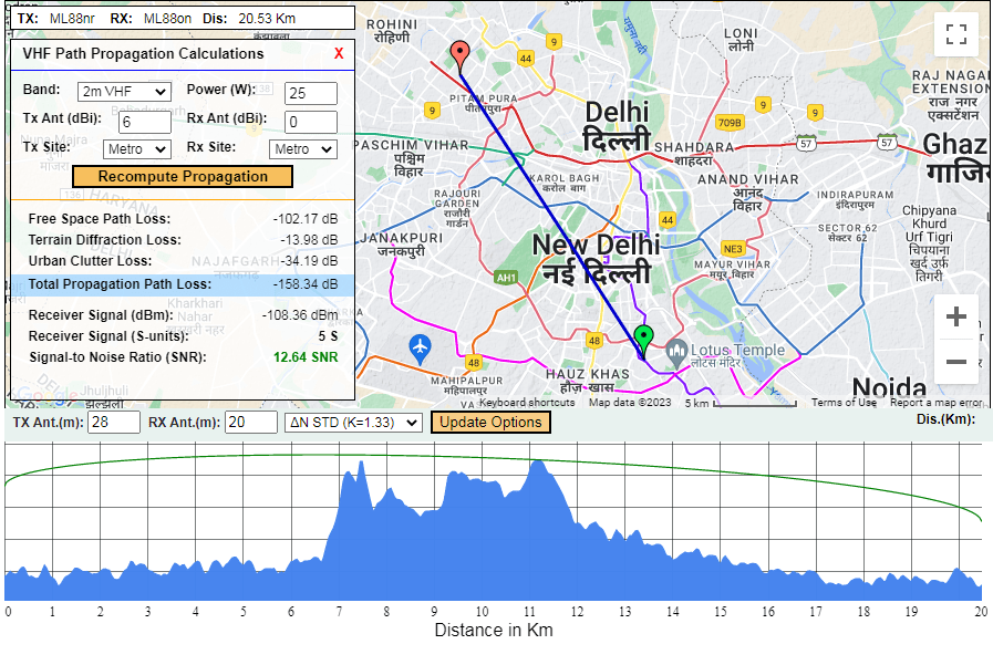
The VHF Propagation Path Profiler TX station conditions have been tweaked adequately to enable a possible communication link between the 2 points. A small increase in TX antenna height and gain did the trick. The available RX end SNR is now acceptable.
The VHF Propagation Path Profiler application allows us not only to trace topological terrain profiles along the communication path but also computes the feasibility of communication over the link and provides us with various signal loss and strength parameters. Not only that, but it also allows us to find alternatives and tweaks that might be needed at the TX and/or RX station setup in terms of TX power or antenna height/gain, etc...
More importantly, the VHF Propagation Path Profiler application provides us the ability to model communication link budgets under different types of atmospheric refractivity gradient (ΔN/ΔH) conditions. For instance, under many long-distance DX communication scenarios, even with all practical enhancement at the TX or RX sites it may still not be possible to achieve viable propagation under the typical standard atmospheric (STD K=1.33) conditions. However, if we try to recompute by setting the atmospheric conditions to different refractivity gradients that allow more signal bending, then communication might become possible.
Experimenting with different Refractivity Gradient Atmospheric Conditions
If despite practical optimized tweaking of TX/RX station parameters it is still not possible under the K=1.33 parameter, one-by-one try to recompute with the next higher K values selected from the dropdown menu. You might find that communication becomes possible at one of these K-value settings. It means that communication across the path is not impossible but will only occur if the atmospheric conditions were such that allow signal bending (via Super-Refraction)... In other words, although the communication link will not be available throughout the year under normal circumstances, it will become viable under certain weather conditions that provide the type and magnitude of refractivity gradient needed to sustain the link.After all, isn't amateur radio all about finding and leveraging elusive propagation openings? We can make VHF/UHF contacts across hundreds or even thousands of Km at times... The VHF Propagation Profiler application can be used to pre-validate prospects of such DX contacts across any two viable locations anywhere in the world.
Those who wish to follow deeper and establish a correlation between K-value and ΔN/ΔH may note the following...
- The equation for converting K-value to ΔN/ΔH is: ΔN/ΔH = 157 x (1 - K) / K
- ΔN/ΔH=-39 for K=1.33
- ΔN/ΔH=-105 for K=3
- ΔN/ΔH=-140 for K=9
- ΔN/ΔH=-148 for K=18
- ΔN/ΔH=-152 for K=35
- ΔN/ΔH=-156 for K=99
- The theoretical Magic Graient ΔN/ΔH=-157
When you discover communication prospects at other higher K values other than STD K=1.33, please remember that the higher the K-value for which your link works the lesser the prospects of encountering applicable weather conditions... For instance, K=3 or K=9 may occur relatively more frequently over the seasons, while higher K=18 or K=35 conditions may be quite rare. The conditions reflecting K>99 may be a once-in-a-blue-moon phenomenon and might occur over a short timespan... Another important factor to remember is that more sustainable higher K value conditions would be more frequent along coastal regions near the coastlines... Experiment and learn!
Intermediate terrain feature visualization
Before we conclude, let me introduce you to another interesting and perhaps under some circumstances also fairly important auxiliary feature of the VHF Propagation Path Profiler application. This is the intermediate terrain feature visualizer function.
After the topological elevation profile chart is generated, some of the topological features of the terrain might be of interest to us. Several specific peaks and valleys along the path may at times be of significance.
For instance, there may be a high hill along the path which might be the cause for considerable diffraction losses across the circuit. We might consider the prospect of using that peak as a possible repeater location. Hence, we need to first identify that peak and find its exact geographic coordinates. We may also like to do a quick visual test on LOS feasibility from the identified hill to either side of the communication path. We should be able to choose between different hilltops in case of multiple hills and thereafter decide which peak might be best suited to meet our objectives. This VHF Propagation Path Profiler application allows us to do just that... Check out the illustration below and read on...
The VHF Propagation Path Profiler application working in Intermediate Terrain Feature rendering mode to allow examination and analysis of intermediate terrain features along the communication path.
Here is the procedure to evaluate and visualize the intermediate terrain features along the elevation profile chart. Roll the mouse pointer across the elevation profile chart and Left-Click on the desired feature. A yellow-colored marker appears at the appropriate location of the blue-colored geodesic path on the map. This marker indicates the geographic location of the terrain feature on the map. The height of the feature ASML can be found from the dynamically updated righthand top end above the chart.
After setting the terrain feature yellow marker on the map, you may roll the mouse pointer over (left-click for touchscreens) the yellow marker. A popup window would open with latitude, longitude, and other information. You may also zoom in and pan the map to inspect the feature closely on the map if you wish. Clicking the mouse on another feature across the elevation chart will shift the yellow marker to its relevant position. The mouseover data of the marker will also get automatically updated.
Once you set the yellow terrain feature marker, you may now left-click on the yellow marker. The color would turn orange and the effective LOS path between the yellow marker location and the TX location will be displayed on the chart. If you click again on the marker then the displayed LOS path will flip to the other side towards the RX location. Subsequent clicks on the orange marker will flip the path rendering between TX and RX sides. Please note that this feature is purely meant for visualization. Therefore propagation metrics computations are not made for these intermediate paths.
When you wish to terminate the visualization mode and revert to the original TX/RX full circuit mode, Double-Click the mouse anywhere on the elevation profile chart area. Control will be returned to the primary regular mode.
After you finish working and analyzing a path if you desire to analyze a new path, you may double-click on the map area and reset the application... You will be ready to start afresh.


(9 votes, Rating: 5.00) - Please vote the article with your valuable star rating. Thanks! Basu (VU2NSB)


SSN SSNf(10.7) – Real-time Solar Data