

Introduction to Radio Communication Noise
After all, what is noise? Is it something characteristically different from the signal? Can the signal be extracted and isolated from the noise by any simple method?… To be able to answer these questions, we need to look deeper into the anatomy of noise.
To begin with, the basic composition of radio frequency noise is no different from the radio signal. They are both electromagnetic waves and they both reside in the common passband that is occupied by the desired signal. So, how do we get rid of the noise? The short answer is that WE CAN’T… However, by understanding the composition of noise, we might find ways and means of mitigating the noise problems by optimizing our communication to favor the signal and not the noise.
The radiofrequency noise may originate from several sources. The importance and relevance of each of these noise sources vary with the portion of the frequency spectrum that we use. For instance, a certain source of noise may be more prominent on VHF/UHF bands or higher, while it may not be of much consequence on HF bands and lower or vice-a-versa.
Some of the contributory noise sources may be in the form of electronic hardware of a radio communication system, whereas, other noises come from extraneous sources. For instance, the earth’s atmosphere produces a considerable amount of static noise, and so do our sun, planets, and other galactic sources. Weather system events like thunderstorms and lightning flashes also add to our woes. These extraneous noises are picked up by the radio communication antenna systems at the receiver end to play spoilsport.
Let us now dwell on the anatomy of the aggregate noise to figure out how to deal with it and optimize our radio communication systems to mitigate their adverse influence. However, we must remember that both our signal as well as the noise are similar in core composition. Hence, once they mix together, it is almost impossible to isolate them using traditional means.
The Basic Anatomy of RF Noise
What is the difference between signal and noise if any? Well! not much at all… Both are electric voltages, currents, or EM waves. Both exist across a common frequency span (passband). They are more or less homogeneously mixed together. The noise and the signal they ride on each other to create an aggregate voltage waveform at the radio receiver front-end.
Having discovered the challenges posed by noise, let us now focus on dissecting the aggregate noise to find its composition.
We noted earlier that primarily, there are two broad noise sources. The one originates from the radio station equipment while the other is extraneous. The extraneous noise may be produced either by nature or it could be man-made.
communication Hardware Noise Sources
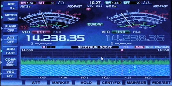
Typical aggregate noise floor as indicted on S-meter on the 20m band.
Although different types of semiconductor material used in the fabrication of transistors or integrated circuits (IC) contribute different quantum to the aggregate thermal noise generated by the electronic circuit, they all have a temperature dependence. The aggregate thermal noise reflected at the input of the radio receiver determines the noise floor of the radio receiver. The noise characteristics of a radio receiver are often designated by Noise Figure (NF) or Noise Factor or at times as the equivalent Noise Temperature.
We discuss receiver noise, noise factor, etc in separate articles under our Radio Rigs section under Communication receivers. For the moment, it will suffice to realize the input noise characteristics of a radio receiver plays a role in determining the limiting noise floor. The higher the ambient temperature of the radio receiver hardware, the higher is the thermal noise produced by it. If many of us were to recall, we might remember that highly sensitive special purpose receivers used for deep-space communication or radio-astronomy almost invariably use receiver front-ends that are operated a cryogenic temperature by colling them with liquid nitrogen, etc.
Natural Noise Sources
Let us take a quick look at the extraneous radio noise sources before we move on to dig deeper. The most prominent contributors are Atmospheric noise, Weather System noise, and Galactic noise. However, thankfully, they do not usually manifest together to batter our radio communication. These noises are largely frequency dependant. The magnitude of aggregate extraneous natural noise is significant at HF while it becomes less at VHF and UHF.Man-made Noise Sources
The other source of extraneous RF noise is man-made noise. As one might expect, typical aggregate man-made noise is maximum in industrial and urban areas which gradually reduces as we shift to the suburban and rural areas. The sources of man-made noise may be quite diverse. The high tension overhead power grid transmission lines generate RF noise and so do automobile ignition systems. Industrial electric machinery, as well as household appliances, are major sources of RF noise. The kitchen appliances like the mixer-grinder, the microwave oven, television receivers, computers, etc among many others all contribute to the aggregate man-made noise.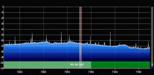
Typical expected Gaussian noise across the band on 40m at mid-latitudes.
Just like any radio emission, the noise is also electromagnetic waves. They too propagate like any radio signal and bear polarization characteristics, This fact brings us to a very interesting behavioral trait of the radio noise in general. Most noise sources produce radiations that are randomly polarized. Hence, the noise energy includes both horizontally as well as vertically polarized components.
Now, here is a fun fact… If we recall the propagation characteristics of short-range coverage, we realize that the major propagation mode of man-made noise will be surface wave propagation. To recap its characteristics, please refer to our article on Ground Wave Propagation. As we learned, the horizontally polarized wave features a far shorter range coverage than the vertically polarized waves. As a consequence, man-made radio noise sources originating from a larger radius (i.e. larger area) around your location (QTH) will reach us if they have vertical polarization rather than horizontal. Although all noise sources generate both polarizations, the net aggregate of magnitude reaching our QTH will be far greater for the vertically polarized components. Actually, the strength of the vertically polarized noise component is so large in comparison to the horizontal that quite often we tend to say that the man-made noise is primarily vertically polarized.
What is the general takeaway from the above discussion? The polarization of our antennas at the radio station often plays a crucial role to determine the magnitude of man-made noise-related woes that we suffer. This is far more true on the HF bands, especially the top bands from 160-40m. This is because the surface wave range coverage is far greater at lower frequencies which leads to the aggregation of noise from many more noise sources within several kilometers around our vicinity. Since the Surface wave coverage is almost non-existent in the VHF/UHF region, most of the noise that reaches our antennas are typically LOS and therefore isn’t much dependent on noise polarization.
Inadvertent Noise Sources
All that we discussed so far is notwithstanding the unfortunate truth that many poorly set up amateur radio stations are often plagued by additional noise being picked up by poorly configured transmission lines and antennas. Improperly set up transmission lines may be prone to noise due to imbalances giving rise to common mode currents. However, that is another story that we will cover in detail in a separate article.Other than this, the station equipment may have poorly set up grounding that creates ground loops that too give rise to elevated noise issues. There may also be near field coupling from various noise sources near the radio equipment or even conducted noise entering through the station equipment power lines. However, we will not expand on these at this point because such noise is entirely different animals and is caused due to poor radio station deployment practices.
After having introduced various probable types of noise affecting radio communication, let us now try to figure out a bit more about them. In the rest of the article, we will focus on HF radio noise because most of the noise types that we discussed so far plague HF radio far more than VHF or UHF. The majority of the noise on VHF and above (for a properly set up station) for terrestrial communication is primarily on account of noise originating within the station equipment hardware. We will dwell deep into those aspects in our section on Communication Receivers.
Analysis of HF Noise Levels affecting Radio Communication
Most of us who work on the HF bands and live in urban and suburban areas do experience S-meter deflections due to static noise as high as S9 or perhaps even more during certain times of the day and seasons on the top bands. Normally, one would expect the static noise floor to be higher as we move down the bands. That is all very true. As we progressively tune up the bands moving to 20m or higher frequencies, we usually experience a sharp drop in the noise floor that results in far lower S-meter noise-based deflection.
The question is, why is it so? Well, let us explore the nature of the atmospheric noise and its characteristics and try to find a correlation to the way mother nature behaves and what the S-meters display.
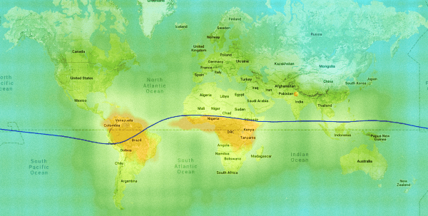
Noise Floor profile across the world due to atmospheric noise on 20m band. (Regions in orange color indicate highest noise levels while yellow, green, and blue indicate progressively low noise levels)
The first one is the noisiness of the operator’s QTH from the perspective of man-made noise. As per CCIR classification, the standard noise level at every location around the world has been set starting from “Very Quiet Rural” to “Suburban“, “Rural“, “Urban“, and “Industrial” environments. This means, for instance, that the local man-made noise levels due to electrical machinery, overhead power transmission lines, automobile ignition, etc are much lower at a rural QTH than what one may expect at a typical modern urban QTH. This man-made noise (QRM) is the primary cause of elevated noise levels on top bands, however, the elevation of static atmospheric noise is also a very significant factor.
Other than the static atmospheric noise that we will discuss in a moment, the important aspect that we should mention at this stage is related to lightning discharges within our atmospheric weather system. Although this phenomenon does not play up consistently, it is also quite important and would be unwise to ignore it.
Typically, the world is witness to about 1.4 billion lightning discharges per annum. All these are not cloud-to-ground strikes, many of them are intra-cloud or cloud-to-cloud discharges. Each of these discharges would prevail with power levels from 40-100 KW. These are like impulse radio transmitters placed at high altitudes. The energy spectrums of these discharges are widespread with decaying amplitude at higher harmonics. Nevertheless, lightning can cause noise interference starting from VLF and all the way up to UHF and lower microwave region.
Ongoing multiple Cloud static discharges and lightning from distant locations produce RF noise energy across the HF spectrum. These noises propagate over distances using the same propagation mechanisms that we use for communication. The noise outputs aggregate and produce random Gaussian noise at our receiving antennas.
The influence of atmospheric weather systems on HF communication is very interesting and has extensive ramifications on HF radio… It would mean variability of noise floor and Signal-to-Noise Ratio (SNR) with the diurnal change, seasons, geo-spatial location of QTH, etc. Operators in the different hemispheres would have different variability of HF noise parameters and hence would have different communication experiences. The regions closer to the Equator will have different effects in comparison to those near the poles. The implications and variation of behavior from one geographic location to another can be mind-boggling.
Let us now commence our analysis below and proceed in a logical manner, step-by-step, and eventually try to present an HF noise model to the readers. Based on various comprehensive CCIR documents, I have created several illustrations in the form of graphs to progressively reconstruct the logical process that would lead to determining the typical aggregate noise floor levels that we might expect across the entire HF radio frequency spectrum. The derivations made in this article are based on CCIR Recommendation ITU-R P.372.8 document for radio noise. We will integrate the effects of various noise sources one at a time and apply them as we progress through our narrative of the noise modeling process.
Static Ionospheric Noise Sources and Composition
This is the fundamental component of atmospheric noise and is derived from the thermal noise generated by the movement of molecules of various gases in the surrounding air. Due to the collision of molecules, kinetic energy is released and converted into a broad spectrum emission of electromagnetic waves. The noise floor is determined by the temperature of the medium. The standard reference temperature for calculating the base noise is taken as 290 degrees Kelvin (°K) which is equivalent to 17 °C.
When a receiving antenna is deployed it picks up this ambient static noise. However, the level of ambient static radio noise at an RX antenna is not frequency independent. There are several reasons for that. One reason is that at lower frequencies the antenna aperture becomes larger and is proportionate to the square of the wavelength. Another reason is that the ionosphere at HF plays an important role in vertically bouncing back noise energy to the antenna thus strengthening it between 2-9 MHz regions. The ionospheric canopy behaves like a curved reflector to enhance the magnitude of the noise at the receiving antenna. There are several other reasons which determine the shape of the atmospheric noise curve.
However, to avoid making this article too technical, we will stop right away and present you with FIGURE-1. This is an ambient static noise curve provided by CCIR. This is the green-colored curve that represents the noise-frequency distribution from 10 kHz to 30 MHz. The noise is presented as “Antenna Noise figure” where 0 NF is equivalent to a noise temperature of 290 °K. you would notice that this ambient antenna thermal noise rises steeply below 1 MHz. Then it rises again after 1.2 MHz till around 9 MHz due to Ionospheric reflection. Beyond 9 MHz, it drops down to reach 0 NF level at 20 MHz… This drop happens due to vertical penetration through the ionosphere.
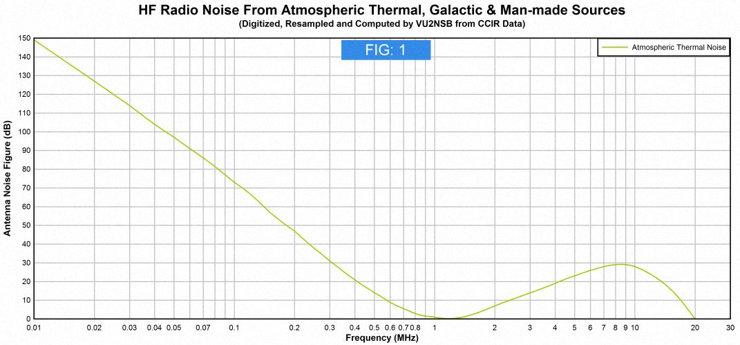
Typical atmospheric thermal noise profile across the VLF to HF spectrum.
Since our frequency range of interest lies in the HF band, let me present FIGURE-2 which is an expanded version of the same curve covering our region of interest from 1-30 MHz.
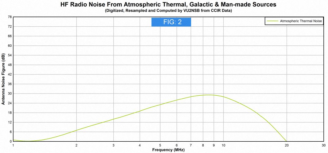
HF atmospheric thermal noise profile expanded to cover the frequency range of 1-30 MHz.
Galactic Noise Sources (Cosmic Noise)
Now, let us bring in the next source of noise which will be instrumental in contributing to our aggregate HF noise floor. This is “Galactic Noise” or cosmic noise. This noise comes from the EM wave radiation from the Sun, planets and various other stars and heavenly bodies in our galaxy. The cosmic atomic and sub-atomic particles from the galaxy as well as solar wind which manage to penetrate the earth’s magnetosphere also contribute to that galactic noise. Like all other natural noise sources, this too has a Gaussian distribution.
FIGURE-3 adds this source to our graph set. The Galactic noise curve is depicted in pink color. The lowest frequency of this curve is curtailed at 6 MHz. In reality, the low-frequency galactic noise limitation could well be as high as 9 MHz. This low-frequency limit is determined by Ionospheric slab density. High Ionospheric density prevents low-frequency galactic noise from penetrating it and reaching the RX station on the earth’s surface. Below the lower side cut-off, the galactic noise cure is portrayed as a horizontal dotted line extension.
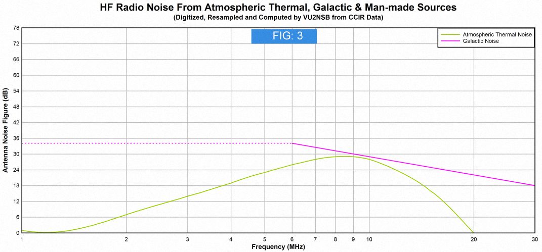
Galactic noise profile added to Fig-2 to show the effects of both atmospheric thermal noise and galactic noise on HF bands
Man-made Noise (QRM) – Sources and Behavior
Man-made noise is a prominent source of noise. This is produced by electrical machinery, home appliances, computers, overhead power lines, automobile ignition, etc. The intensity is highest in Industrial and Business districts followed in descending order of intensity by Urban residential complex, suburban locations, Rural, etc. The noise power density of this kind of noise is higher at lower frequencies and gradually decreases in the upper HF region. FIGURE-4 shows several types of man-made noise density curves. The blue color lines on a logarithmic frequency scale have been added to this figure. The dot-dash line and the dashed lines represent Business Area noise and Quiet Rural Area noise levels respectively.
The lines for Urban and suburban areas would fall in between these lines. The overall radio noise floor will eventually be determined by the level of man-made noise at any specific geographic location. Rather than attempting to complicate our narrative by determining the overall noise expected to prevail under various different conditions of man-made noise environments, we will choose a single scenario. Once I explain the process of determining expected noise levels, the reader can easily extrapolate to find noise levels under different QRM conditions.
Let us choose the “Very Quiet Rural” location scenario to continue this discussion, while the other QRM level scenarios would be ignored for now. We will use the SOLID BLUE line in our computations because it represents the “Very Quiet Rural” location which we chose to factor into our presentation. From these lines (curves) you can get an idea of how man-made noise contributes to the overall noise scenario.
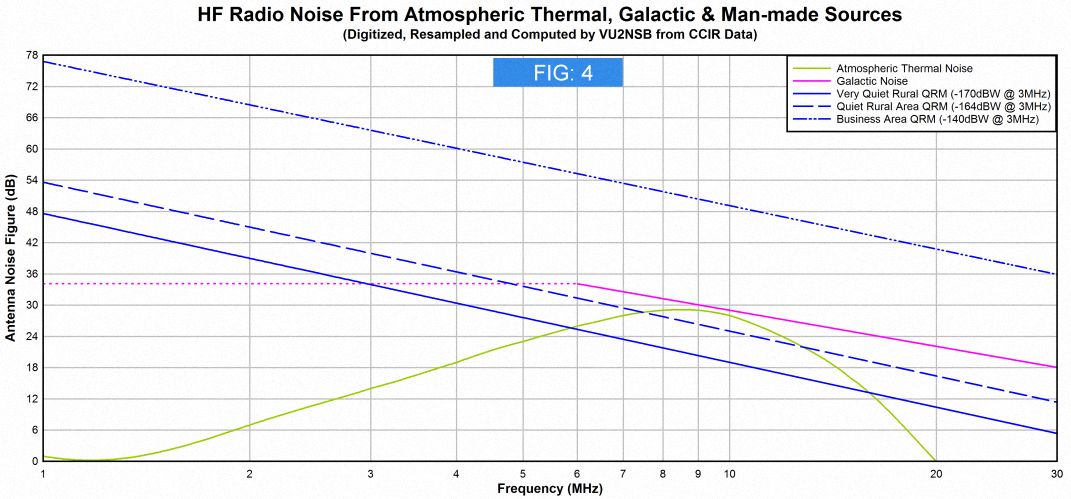
Man-made noise levels (QRM) added to Fig-3 to show effects of atmospheric noise, galactic noise, and man-made noise levels across the HF radio spectrum.
Total Combined Effective HF Noise
To determine the combined Effective HF Noise Floor, we will now combine by adding the noise produced by the three above-cited sources.
- Atmospheric Thermal Noise (Green).
- Galactic Noise (Pink).
- Man-made noise at a quiet rural location (Solid Blue).
Since all the three noise sources are presented as Noise-figure NF (dB), we will perform a logarithmic addition of all the three curves across 1.8-30 MHz (160-10m band coverage). FIGURE-5 shows this aggregation as a thicker red-colored trace. This is the final analytically derived noise floor on HF bands based on CCIR observations.
I have added an S-unit scale that correlates to the NF scale on the left side. This is to make it easy for the reader to correlate the projected noise levels in S-units.
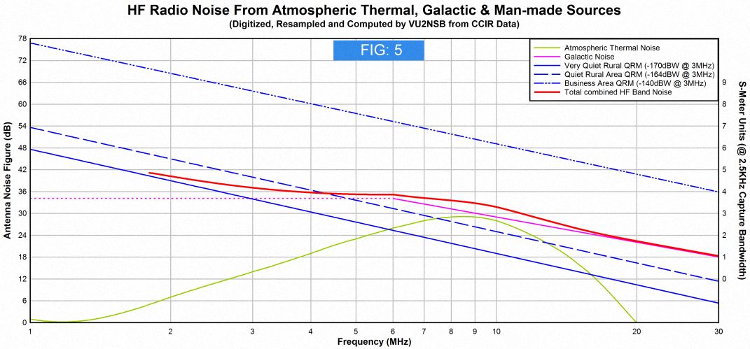
Aggregation of the effects of all discussed noise sources have been displayed here. The aggregate HF noise floor spectral graph considering Very Quiet Rural QRM level conditions is shown by the bold red curve.
Although, in our discourse, we chose to use the man-made noise levels prevalent at Very Quiet Rural (-170dBW @ 3MHz noise) location to magnify the contributory effects of other noise sources like the atmospheric noise and the galactic noise on the aggregate curve (Red-colored curve) shape, it would be more realistic in the real world to factor in higher man-made noise levels that might fall between the Rural and Industrial noise levels. Typically, a QRM level that is 12-18 dB higher than what is used in this example scenario should be quite real. The net result will be to elevate the combined aggregate noise curve by 2-3 S-units at low and mid-frequency portions of the HF spectrum. In that case, one will find that the noise floor levels on the 80-40m band segment might turn out to be about 6-7 S-units. Of course, many urban and metropolitan operators may sometimes experience even a higher noise floor on the 80m band especially near the equatorial region.
Please note that in this article I have considered typical average atmospheric thermal noise levels and ignored the effects of diurnal, and seasonal variations. These factors play a role too but accounting for these factors is beyond the scope of this article. However, I will take these up in detail in subsequent articles under this section.
- Most noise sources have wide frequency spectrum and have a Gaussian distribution.
- Atmospheric noise is perhaps the most significant element of HF band noise.
- Low latitude locations near the equator are more prone to a higher magnitude of HF band atmospheric noise.
- Earth’s weather system is often responsible for elevating noise levels during thunderstorms and lightning.
- Galactic noise sources affect HF bands marginally but it is most significant on VHF or above.
- Man-made noise is dominant in urban areas and causes a big challenge to top band HF communication.
- The aggregate magnitude of vertically polarized man-made noise is far higher than horizontally polarized noise.
- Vertically polarized HF antennas are prone to produce greater noise at receiver input than horizontally polarized antennas.


(30 votes, Rating: 5.00) - Please vote the article with your valuable star rating. Thanks! Basu (VU2NSB)
SSN SSNf(10.7) – Real-time Solar Data


