Do we need to set eaxct antenna bearing for HF DX?
Of course, what we are discussing here is notwithstanding the fact that for VHF/UHF terrestrial radio contacts across several tens of kilometers one would need to beam quite accurately. Not only because the beam flare-out is narrow at short distances but also because much higher antenna gains on VHF and beyond produce far narrower beams… However, right now, we concern ourselves only with HF antennas for DX contacts.
People at times ask me, What is your Grid-square? or, I only copied VU2N?? what is your full callsign? Unless I know it, I can’t decide where to turn my beam. I need your full call to look up the beam heading to swing my antenna to you… and so on so forth…
So, Why all this confusion?
All this makes me wonder, where does the problem lie? Why would anyone want to compute the exact beam heading to my QTH for an efficient HF radio QSO? To reach me, an approximate intuitive orientation of the antenna heading towards South Asia from any DX location should be more than sufficient for a long-distance HF contact. Does anyone really need to know my whereabouts more accurately? The answer to all this is a definite NO. Unless we are located less than 3000 Km or more than 17000 Km apart. Barring these two unique scenarios, normally for working DX between 3000-17000 Km one can relax and take it easy.
Communication at short distances
At distances less than 3000 Km the antenna beam flare-out is limited. Hence one might need to know where the other station is located with a little better precision. Normally this should not be a cause for worry because anyone would probably know the geographical layout around his QTH fairly well. For instance, anyone living in Frankfurt, Germany would know that Prague is due East, Amsterdam is North-West, Paris is almost South-West, Copenhagen is a little East of North, Zurich, and Milan are due South, etc. It is all simple neighborhood geography. The Great Circle paths at short distances are essentially straight lines.Communication close to Antipode distances
However, at distances beyond 17000 Km, it is an entirely different 3D Spherical Geometry phenomenon. It happens on account of antenna beam convergence at the antipodes of the nearly spherical earth that has a nominal perimeter of around 40000 Km. Hence the antipode is at nearly 20000 Km, which is half the perimeter length. Antipodal convergence has many interesting effects which we will perhaps discuss separately in another post or a full-fledged article. However, you may check out our brief post Challenges of working HF DX near Antipodes in the meanwhile. Within the scope of our discussions here, we will try to explain that by and large, for HF DX up to distances of 17000 Km we need not be touchy and finicky about our HF antenna beam headings.On many occasions, I come across operators who are very concerned and perhaps feel a little lost since they would not know the exact beam heading to a DX location. They waste a lot of time trying to find out the Grid Square or Lat/Lon of the DX. Knowing the Grid Square of the DX station is not necessary unless you have no clue as to where on earth (both literally and figuratively) his country is located. All that one needs to do is to brush-up some basic geography and the concept of Great Circle Maps and paths. We don’t need anything beyond this to work effectively on HF radio from the perspective of the determination of antenna heading. We will discuss Great Circle Maps (GCM) under our website section on Geodesic for Terrestrial HF Radio. At present, the issue that I am trying to highlight is more fundamental.
Typical misconceptions and their explanations
Quite often I have had stations responding to my CQ call but was unsure which way to beam their antenna. For instance, at times a station would be loud and clear with say S7-8 at my end. He would tell me that he is beaming at 90° towards me from Europe. Then he would ask for my Grid Locator. I would oblige to his request but ask him not to bother as long as he is beaming into India or perhaps broadly into any part of South Asia. In the next round he would come back and tell me that he had a wrong beam heading and now since he discovered it, he corrected it to 87°. Hence he would want another signal report. Unfortunately, to his dismay, my report would still be the same. A small 3° azimuth swing of his beam made no perceptible difference. He would be more confused and wonder if something was wrong.
Well, nothing is wrong with anything, for that matter, nothing is wrong with either him or me. Everything is perfect and normal. While working on HF with practical directional antennas we need not be concerned about the precision of beam heading. Almost all directional HF antennas barring a few like the very long traveling-wave antennas (Beverage or Rhombic) or big stacked arrays with significant horizontal stacking, all other antennas have a fairly broad beamwidth. For instance, a 3-element Yagi would have ±40° azimuth beamwidth, while a big 8-element high gain Yagi too will have around ±28° beamwidth. All other antennas whether a Cubical Quad or LPDA or whatever, a mono-bander or multi-bander will have azimuth beamwidth typically from ±50° to ±25°. More likely to be near the higher end of the width for most amateur radio antenna installations.
These beam widths are colossal. As the RX station is further and further away from the TX station, the width of coverage on the map in terms of beam footprint becomes wider. It is like a triangle (or cone) with a wide apex angle. As the distance from the apex increases, the coverage area flares out in width. Simple school geometry used to calculate the base of a triangle with a known height and apex angle will clear the picture. However, on a nearly spherical object like the earth, the surface geometry introduces an important variant. The area coverage due to the beam flare-out is maximum at half the antipode distance of 20000/2 = 10000 Km. After the 10000 Km distance, a geometrical convergence begins to happen till a total convergence occurs at the antipode.
Since illustrations are often worth a thousand words, I will add a few illustrations below which will allow us to visualize it. Based on their beamwidth specifications, the antenna beams flare-out covers increasingly large areas on the map as the distance from the TX station increases. These illustrations will also show you that the flare-out (coverage) is widest at a distance of approximately 10000 Km away from the TX antenna. Beyond 10000 Km a gradual convergence would begin to take place. However, it will maintain a reasonably wide flare-out until about 17000 Km, beyond which a rapid convergence will happen till full convergence occurs at the antipode (approx. 20000 Km away).
Illustrative examples of typical scenarios
Scenario #1 – 8-element Yagi (relatively rare on HF)
This the azimuth beam flare-out pattern for an 8-element Yagi located in New Delhi, India. The blue-colored sector area represents the -3dB beamwidth coverage footprint. The coverage footprint widens and spreads out as it passes through Europe. Although the propagation direction is a straight line around the globe, the rectangular map we are using (Mercator Map) shows the world as a skin laid out in a 2D plane, the straight line around the globe appears as a curved (semi-sinusoid) line which appears to bend downwards.Furthermore, the Mercator map projection is a cylindrical Constant-North Conformal projection used primarily for navigation but also extensively used for plotting Geodesic paths of antenna beams, the way we do quite often for amateur radio purpose. This type of map has the drawback that it distorts and increases the projected size of land masses as we move from the equator to the poles. Hence upper Northern latitude territories like Greenland, etc appear to be larger and vertically elongated. Our antenna footprint flare-out also appears accentuated on the higher side due to this reason.
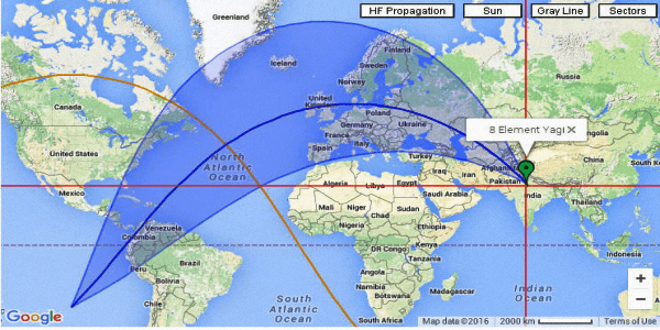
Typical azimuth beam of an 8-element Yagi antenna with projection of the beam flare-out on a world map.
In the blue-shaded antenna beam footprint, the central dark-blue line represents the actual beam heading angle which has been set to 320° from the New Delhi QTH. The footprint flare-out finally converges at a point in the South Pacific. This is the antipode of my QTH in New Delhi and is located at a 20000 Km distance. The orange-colored curved line that you see passing through Canada and then down through the Atlantic is the 10000 Km equidistant line from New Delhi.
We can clearly see that even a narrow azimuth beamwidth antenna like an 8-element HF Yagi has such a broad coverage at DX distances. It becomes practically unnecessary for me to worry about pointing my antenna carefully toward any grid-square. As long as I know my basic geography and where on the map a continent or a country lies, I need to know no more. Just by beaming roughly at 320° (as in this case), I can work the whole of the EU without bothering to move my 8-element Yagi beam.
Scenario #2 – 3-element Yagi (Most common HF Beam Antenna)
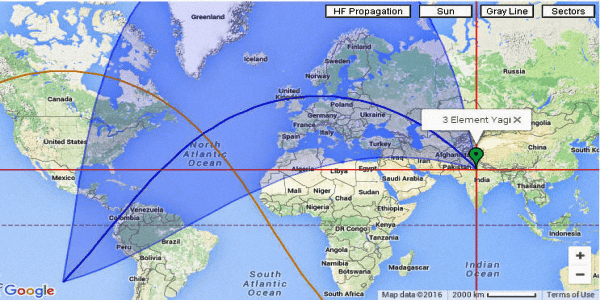
Typical azimuth beam of a 3-element Yagi antenna with projection of the beam flare-out on a world map.
This is the same as above in all respect but represents a 3-element Yagi once again beaming at 320° from my QTH at New Delhi… This antenna has lower gain and hence a wider beamwidth. Since the azimuth beamwidth is wider, the antenna footprint flare-out is also wider. Hence the territory covered by a 3-element Yagi is bigger. Without altering my heading not only can I can easily cover the entire EU, but also most of middle-east, Central America, the Caribbean, some northern parts of South America, and most significantly large parts of inhabited Canada, the US east coast, and parts of north-east and the central USA. I do not need to swing my beam around to cover all these places.
Scenario #3 – (Cardiod Pattern representing wide Beam)
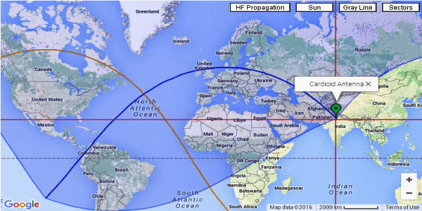
Typical azimuth beam of a Cardioid pattern antenna with projection of the beam flare-out on a world map.
The third illustration represents an azimuth beam flare-out footprint for a Cardioid Pattern Antenna. This antenna pattern nearly represents a large variety of real-world amateur radio antennas that usually produce very wide azimuth patterns which may at times be bidirectional too. In this case, too, the beam heading for the antenna is at 320° as in previous illustrations and also located at a TX site in New Delhi, India. Due to the very wide beamwidth of this antenna which is in excess of 180°, it covers one full hemisphere at a time without your having to swing the antenna. With the current beam heading of 320° from New Delhi, as seen in the picture, I successfully cover all places on the globe except VK/ZL land, South and South-East Asia, the lower half of Africa, and Southern tip of South America.
A Wrapup of Conclusions and Key Takeaways
We discover that while working with HF radio, we need not really be worried about our exact and accurate beam headings. The azimuth beam flare-out is quite wide with all practical antennas that might be available to us on HF bands. Even a relatively narrow-beam antenna like an 8-element Yagi (not used by many due to its sheer size on HF) also has a fairly wide flare-out footprint.
Though I have referred to map projections like GCM and Mercator in this post, detailed discussion on types of Map projections is beyond the scope of this post. However, as I mentioned before, I will take it up in another article at a later date.
In view of the above, there is no point in being very finicky about the precision of the beam heading to a DX location. It is only a waste of time and serves no practical purpose. The only exception would be in a case where the DX station is almost uncopyable and his signal is skimming the noise. This is when perhaps even an additional 1dB would make a difference between a no QSO and a valid QSO. Barring this extreme situation, I would suggest that one should take it easy and not be too worried about heading precision.
I personally never bother about the last digit of the azimuth value even on a rotator with a digital display… On the 0-360° scale, I mentally use the least count of 10° or even 20° depending on the antenna I use. As long as my beam heading is within 10-20° of the theoretical value, I am least concerned. Quite often I go a step further. From my QTH in New Delhi India, whenever I work Europe, I beam roughly into the central EU and forget about it. If I find band openings into East and Central parts of North America, I just swing my beam a little further north, perhaps into Scandinavia or the Baltic Sea. This way, not only do I continue to work the entire EU but also NA including Central America and the Caribbean. Similarly, if I need to work VK/ZL land, I swing my beam coarsely anywhere into central Australia. This way I get full coverage of Southeast Asia, Australia, New Zealand, and the entire Oceania region.
To summarize, I would say that we really do not need to be unduly worried about the accuracy or precision of our antenna beam headings. Antenna beams are like broad flashlight beams. Further the object to be illuminated by the flashlight; the broader will be the area of illumination. It is not like a Laser beam and you do not need to point your antenna towards the DX like a sniper rifle…
Happy DXing es 73, de Basu (VU2NSB)

Contents

(11 votes, Rating: 5.00) - Please vote the article with your valuable star rating. Thanks! Basu (VU2NSB)


Ham Rig Reviews Coming Soon
SSN SSNf(10.7) – Real-time Solar Data