Do Digital Modes like FT8 work Below Noise?

December 26, 2019 | Author Basu (VU2NSB)

Digital modes like FT8 work below Noise? – A myth

It is a common myth that narrowband digital modes like FT8, JT65, etc establish communication with signals that are below the noise floor. This myth has by and large been perpetuated among the amateur radio community where many operators consider it to be a magical property of these digital modes. These narrowband digital mode signals may not be audible on a regular radio receiver or may not be visible on the band-scope spectrum or waterfall displays of our transceivers but there is nothing magical about it. They certainly do not work with signals being below the noise floor.

Barring a few modulation modes like the Spread Spectrum, including both direct Sequence Spread Spectrum (DSSS) and the Frequency Hopping Spread Spectrum (FHSS), typically most other commonly used digital modes need signals to be above the noise floor with a positive magnitude of Signal-to-Noise Ratio (SNR). Spread Spectrum due to its nature, has a very low signal density that typically lies below the noise floor. Hence, it is difficult to detect and equally difficult to decode. This is the reason why authorities around the world are wary of allowing radio amateurs to operate Spread Spectrum… But that’s a story for another day.

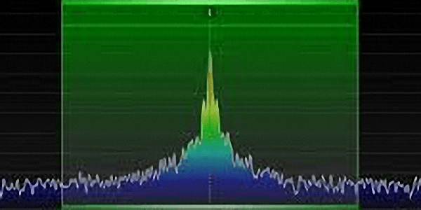
A typical Communication Receiver – Noise vs Signal

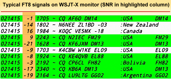
A screengrab of typical SNR levels (Relative to 2500 Hz receiver detection bandwidth) reported on a FT8 monitor. Note that the SNR values are all negative indicating signals to be below the noise.

A typical communication receiver or a transceiver hat we use for amateur radio is designed to cater to SSB radiotelephony, CW, and various other forms of digital communication including analog and digital SSTV. The primary filter bandwidth of the receiver chain is typically designed to process signals with up to 2500-2700 Hz baseband channel bandwidth. This filter bandwidth also determines the receiver bandwidth or what is called the Detection Bandwidth in technical terminology. Of course, we also have options to switch in narrower bandwidth filters to cater to a better CW experience. However, even with the CW filters switched in the channel bandwidth is usually no less than 250-500 Hz. Even this is far too wide for optimum narrow-band digital text modes.

When tuning across the band to locate signals, it is a usual practice among radio amateurs to select the SSB filter (~ 2500 Hz). This allows listening to various types of signal modulations with ease. Under these circumstances, various narrow-band digital mode transmissions like PSK, MFSK, JT9, JT65, FT8, WSPR, etc may not be audible or not be visible on the band-scope or waterfall displays of the transceiver. Yet, these signals can be copied and perfectly decoded by various software utilities designed to decode these digital modes.

Why is it so? If the digitally modulated transmission is inaudible and below the noise floor, is it not logical to conclude that these didi-modes work well with negative SNR? The answer is an emphatic NO… This brings us to the concepts of Noise bandwidth and Modulation bandwidth. Let us see what they are.

The concepts of Modulation and Noise Bandwidth

A typical narrow-band digital signal passing through a detection window with a wide noise bandwidth eventually resulting in the notion of a negative SNR with signal below noise.

Let us first briefly figure out the Modulation Bandwidth of a modulation mode and thereafter correlate it to the Noise bandwidth of the communication channel. This will provide us an insight into what is really going on. We have a separate article on this subject which goes into the details of noise bandwidths under the section on Noise in Radio Communication that you could read later.

Modulation Bandwidth

Different types of radio signal modulations have different modulation bandwidths to carry information. For instance, a typical SSB modulation bandwidth for radiotelephony is around 2500 Hz, while normal CW may require 100-250 Hz bandwidth depending on the keying speed. On the other hand, digital text modes like PSK31 (BPSK31) at 31.25 bauds (~50 WPM) would theoretically need 63 Hz bandwidth, while JT9, FT8 or JT65 operating at very low baud rates need as low as 1.5-6 Hz only. Lower the information transfer rate (Data rate), the lower is the required modulation bandwidth.

Noise Bandwidth (Detection Bandwidth)

Intuitively, we all know that the background radio hash noise that we hear on HF radio determines our ability to copy a DX station. Greater, the background noise, the more difficult it is to copy a weak station. We also know that when we switch in a narrower receiver filter, the intelligibility becomes better.

The quantum of aggregate noise on any radio receiver frequency is directly proportional to the width of the filter. The wider the filter bandwidth (detection bandwidth), the greater is the aggregate noise. Every time we double this bandwidth, the noise floor power level in the receiver doubles and vice-a-versa. Hence, the signal level being constant, each time we double the receiver detection bandwidth, we increase the noise power in the receiver chain by +3 dB and consequently degrade the SNR by -3 dB, and so on.

This brings us to a vital question… How do we reduce this background noise? The answer is to use narrower filters to ensure narrower detection bandwidths. How narrow a filter bandwidth can we use? This is where we come to the point where we would say that for optimum communication, we need the detection (filter) bandwidth of the receiver to correspond to the modulation bandwidth of the digital mode that we are using. Unnecessarily wide detection bandwidth would result in degradation of SNR which might make the signal not only inaudible but also produce a negative SNR. A perfectly copyable narrow-band modulated digital signal which actually has a healthy positive SNR when copied on a receiver with an optimally narrow detection bandwidth, will appear to have a negative SNR on a typical amateur radio transceiver.

Why do they say that FT8 or JT65 can copy at -26 to -30 dB SNR?
Actually, they don’t… The way it is put across may be quite deceptive and may appear to be misleading to an average amateur radio operator. As I mentioned earlier, all these seemingly magical modes too require a healthy and positive SNR to be able to decode, just like any other modulation including SSB radiotelephony.

This is where we will now revisit the concepts of the receiver bandwidth, filter bandwidth, or detection bandwidth, whatever we might like to call it.

The confusion is because all the negative values of SNR that we find associated with these apparently magical digital modes are all referenced to a typical transceiver setup for SSB with a reference detection (noise) bandwidth of 2500 Hz. If we were to translate each of these negative SNR values associated with such modes to the equivalent required detection bandwidths corresponding to those modes, all the apparent magic will disappear in thin air… Let us unravel the mystery with a typical example below.

Although the real Noise bandwidths for modes like JT9, JT65, and FT8 are approximately 1.7, 2.7, and 6.2 Hz respectively, for the sake of simplicity let us assume the mode in our example has a noise bandwidth of 2.5 Hz. Let us also assume that our example mode needs a positive SNR of at least +6 dB to properly decode the signal with very few errors.

Here are some of the facts…

Signal (or noise) bandwidth – 2.5 Hz
Required SNR – +6 dB

Enhanced Noise floor level, when copied on a typical SSB receiver with 2500 Hz detection bandwidth, will be…

30 dB = 10 x Log(2500/2.5)

The magnitude of the noise floor level is now 30 dB higher in magnitude when demodulated over the 2500 Hz filter window of our receiver than what it would have been if demodulated with an optimum 2.5 Hz bandwidth. We now have a scenario where the noise passing through along with the desired signal into the demodulator would completely drown the signal.

That is precisely what happens. Due to the 2500 Hz reference filter bandwidth of our typical SSB receiver, the SNR as perceived at the receiver output appears to be degraded by 30 dB.

SNR_(2500Hz) = SNR_(2.5Hz) – 30
— OR —
-24 = +6 – 30

What we have seen above is that the signal which actually has a +6 dB SNR when referenced to the mode’s optimum detection bandwidth of 2.5 Hz, now, appears to have a -24 dB SNR when we reference it to 2500 Hz detection bandwidth of our typical radio transceivers. We will see later down this narrative that the software utilities like FlDigi, WSJT-X, etc that we commonly use actually run the -24 dB SNR signal through a narrow 2.5 Hz filter to recover the actual SNR of +6 dB as in this example. Thereafter, the software decodes the +6 dB SNR signal to produce text output.

Therefore, since we can decode the signal nicely under the above conditions, we usually say that this digital mode can be copied at -24 dB SNR.

It is quite convenient to express the weak signal performance of such digital modes in the above manner. It perhaps creates a slight delusional sense of achievement since it often makes an average amateur radio operator believe that he can actually work signals with deeply negative SNR that are drowned deep in the noise. The truth is far from what they might believe.

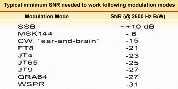
A comparative table of several narrow-band digital modes plus CW to provide a general idea of their weak signal capabilities. All SNR values are referenced to 2500 Hz noise window.

OK, if what you say is true, then how come we manage to decode these signals when our transceivers have wide detection bandwidth and drown the signal in noise?… Fair question!!!

The answer is that our transceivers are generally incapable of directly decoding such signals at all without the assistance from outboard narrow bandwidth signal processing systems or software. The output of the transceiver audio that contains noise across the 2500 Hz bandwidth plus the signal that is sunk well below the noise level is fed to external hardware or software-based decoder. Most often we use software decoders running on our personal computers that are connected to the transceiver.

The wideband noise plus signal that is inputted to the decoder is made to pass through a narrow band filter with a noise bandwidth of 2.5 Hz. The signal that is 2.5 Hz wide stays intact while the excess noise around it is now filtered out. As a result of this, the noise magnitude at the output of the software DSP-based filter reduces by 30 dB (Log(2500/2.5)). Hence, we succeed in reclaiming the original SNR of +6 dB after this elaborate software-based filtering process. Thereafter, the rest of the software decodes the +6 dB SNR signal to complete communication.

The bottom line is that these digital modes do not work magically with negative SNR. The actual positive SNR is cloaked by the way we usually specify it with reference to 2500 Hz bandwidth. The method of specifying SNR of various modes against a 2500 Hz detection bandwidth reference is practical and convenient for the scientific community and all others who are technically minded. It allows easier assessment of relative performance characteristics of various narrowband digital communication modes. However, among a large section of the amateur radio community, it spreads the shenanigan that these digital modes have magical properties of working effectively with signals far below the noise floor.